Background
Nowadays, there is great interest in interventional cardiology and in the medical scientific community in general in the development of prognostic models in the context of survival analysis. In particular, physicians have a variety of tests and biomarkers at their disposal to aid them in optimising medical care, and in many cases these tests are performed regularly in time to provide a better picture of the disease progression of a patient.
When it comes to the statistical analysis of this type of data we need to pay particular attention to the fact that we have two types of covariates/predictors to consider, i.e., covariates whose values are fixed from baseline to the end of the study, and covariates whose values change during follow-up. Statistical analysis of the second type of covariates can prove challenging due to the special characteristics these covariates have, namely that measurements on the same patient are correlated and that very often, based on the values of these covariates (e.g., when a biomarker exceeds a specific threshold), it may be decided that patients need to be excluded from a study (informative censoring). Motivated by this context the aim of this paper is to explain the challenges in time-varying covariates and how analysts should approach them in practice.
As an illustrative example we will consider data from a study conducted by the Department of Cardio-Thoracic Surgery of the Erasmus Medical Center in The Netherlands which includes 286 patients who received a human tissue valve in the aortic position in the hospital between 1987 and 20081. Aortic allograft implantation has been used for a variety of aortic valve or aortic root diseases. Initial reports on the use of either fresh or cryopreserved allografts date from the early years of heart valve surgery. Major advantages ascribed to allografts are their excellent haemodynamic characteristics as a valve substitute. A major disadvantage of using human tissue valves is, however, their susceptibility to tissue degeneration and the subsequent need for reinterventions. Re-operations on the aortic root are complex, with substantial operative risks, and mortality rates in the range of 4-18%1. In this study, a total of 77 (26.9%) patients received a subcoronary implantation (SI), and the remaining 209 patients a root replacement (RR) with an allograft. These patients were followed prospectively over time with annual telephone interviews and biennial standardised echocardiographic assessment of valve function until July 8, 2010. Echo examinations were scheduled at six months and one year postoperatively and biennially thereafter, and at each examination echocardiographic measurements of aortic gradient (mmHg) were taken. By the end of follow-up (median 3.75 years; IQR 5.87 years; total number accumulated person-years: 2,935), 1,241 aortic gradient measurements were recorded with an average of five measurements per patient (SD 2.3 measurements), 59 patients had died, and 73 patients required a re-operation on the allograft.
Types of time-varying covariates
Before we introduce the statistical tools we have available for measuring the effect of time-varying covariates, we should first distinguish between two different types of such covariates, namely, external or exogenous covariates and internal or endogenous covariates. The reason it is important to make this distinction is that endogenous covariates require special treatment from a statistical analysis point of view compared to exogenous ones.
Definition
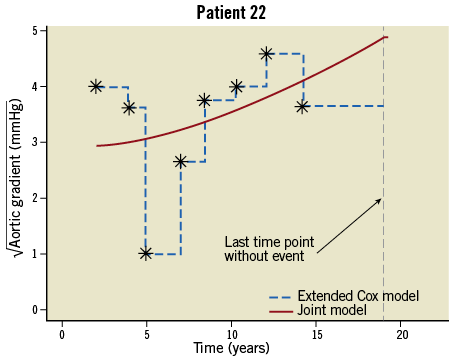
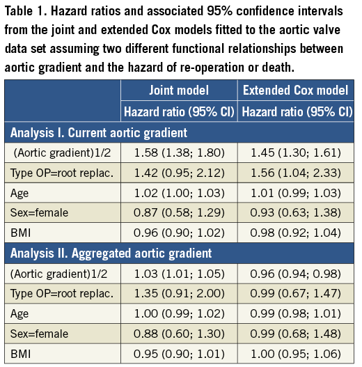
A time-varying covariate is exogenous if its value at any time point t is not affected by an event occurring at an earlier time point s Examples of exogenous covariates are the nurse who took the blood sample or performed the echo, the period of the year (e.g., winter versus summer) and environmental factors (e.g., pollution levels). On the other hand, all covariates measured on the patient, e.g., biomarkers, are endogenous. To make this distinction clearer let us consider two time-varying covariates in the context of our motivating study, namely the aortic gradient levels which have been measured during follow-up and the nurse/physician who recorded the measurement. Suppose that for a particular patient re-operation is required after s=5 years from the initial valve replacement. It is directly evident that at a future time point, say t=5.2 years, the level of aortic gradient will be affected by the fact that this patient underwent re-operation, whereas the choice of which nurse (from the ones assigned to this study) will measure the aortic gradient at the same time point t=5.2 years will not be affected by this re-operation. The next section explains in detail why it is important to make this distinction for the statistical analysis of such data. Methods for survival analysis with time-varying covariates The standard statistical tool which is used to analyse survival data is the Cox regression model. In its basic form we assume that the hazard depends only on covariates whose value is constant during follow-up, such as age at baseline, sex and randomised treatment. When there is interest in investigating whether time-varying covariates are associated with the risk for an event, the extended Cox model can be employed2. This is, in fact, a version of the standard Cox model which can handle both baseline and time-varying covariates, and is available in most standard statistical software packages. However, unfortunately, this extended Cox model is only theoretically valid for exogenous time-varying covariates, and it is not optimal when it comes to studying repeated measurements of biomarkers or of other patient parameters3,4. The reasons behind the inadequacy of the Cox model are best explained via Figure 1 which shows the aortic gradient measurements of one patient from the aortic valve data set. As can be seen, the Cox model assumes that from one visit to the next the marker’s level remains constant, and then a sudden change in the levels of aortic gradient occurs on the day the patient comes to the study centre to provide a new measurement (Figure 1, dashed line). It is of course evident that such an assumption is quite unreasonable for a biomarker. In particular, we expect aortic gradient, and patient parameters in general, to change continuously over time, as the condition of the patient also changes. Treating an endogenous time-varying covariate as an exogenous one and just fitting the extended Cox model would result in bias for the estimated effect of this covariate5 (i.e., effects are estimated as smaller than they truly are), and eventually mask its true predictive ability. We should mention that, even though some refinements of the extended Cox model have been proposed in the literature to settle some of the aforementioned issues, these have not been completely resolved within the framework of Cox models6. Figure 1. Graphical representation of the conceptual differences between the extended Cox model and the joint model. An alternative statistical modelling framework which addresses these issues is the framework of joint models for longitudinal and survival data3,4,7. This is a relatively new and fast developing field of biostatistics research which has shown very promising results in the analysis of serial biomarker measurements8-14. The basic intuitive idea behind joint models is to combine the Cox model with a mixed-effects model. Mixed-effects models are a class of statistical model that is used to analyse correlated repeated measurements data, such as the aortic gradient levels measured repeatedly over time for the same patients in our study population. The appealing feature of these models is that they estimate the biomarker profile over time of each individual patient (Figure 1, solid line). Following on from the previous discussion, this makes more sense from a biological point of view compared to the extended Cox model, because these models explicitly postulate that biomarker levels evolve smoothly over time and do not remain constant between visits. Additional advantages of these models are that they can work even when measurements of the patients have not been taken at the same time points, and that missing biomarker measurements are automatically handled under the missing at random assumption (i.e., the reasons for a missing measurement may depend on previous observed responses, e.g., the physician decides to exclude a patient from the study when the biomarker exceeds a specific threshold). To illustrate the virtues of joint models versus the traditional Cox models, we compare the two models in two different analyses of the aortic valve data set. In particular, an important aspect when modelling time-varying covariates is the functional relationship between the covariate and the hazard of the event of interest. By functional relationship we mean the exact specification of which of the past values of the biomarker up to any time point t are associated with the hazard at t. In general, there are several options for specifying this relationship and its appropriate form and, in many cases, it is challenging to find. For our illustrations we consider two functional relationships, namely, in Analysis I we postulate that the hazard of re-operation or death at any time t depends on the square root transform of aortic gradient at the same time point, whereas in Analysis II we postulate that the hazard at time t depends on the area under the longitudinal profile of each patient up to t. The square root transform was used because on the original scale aortic gradient has a skewed distribution, whereas on the transformed scale the distribution is much closer to normal (decision based on a Q-Q plot). In plain words, in Analysis I we study how strongly associated is the current value of aortic gradient to the hazard, while in Analysis II we study the aggregated effect of aortic gradient to the hazard. In addition, both analyses have been corrected for type of operation, age, sex and BMI. In the appendix we provide syntax for fitting joint models in the R statistical software environment using package JM15 (Online Appendix). Results The results under Analyses I and II are presented in Table 1 which shows hazard ratios and the corresponding 95% confidence intervals under the joint model and the time-varying Cox model for each of the two analyses. We observe that there are differences between the two modelling approaches, which are more evident for the effect of aortic gradient. In particular, under Analysis I and as is medically expected, both the joint model and the Cox model show that increasing aortic gradient is associated with an increase in the risk for re-operation or death. However, we note that, as explained earlier, the Cox model underestimates the strength of this association. Under Analysis II we observe more prominent differences, with the time-varying Cox model showing an opposite relationship to the one expected, namely that, if a patient on average had higher aortic gradient levels compared to another patient up to a particular follow-up time, then the former patient has a lower risk than the latter. This unusual result can be explained by the fact that the ordinary Cox model does not appropriately account for the endogenous nature of aortic gradient. The results from both analyses are in line with theoretical work and simulation studies3,4,14, and convincingly demonstrate that appropriate modelling of serial biomarker levels is required to measure accurately how strongly a biomarker is related to the event of interest and also reveal its true potential for prediction. Conclusions and recommendations An inherent characteristic of many medical conditions is their dynamic nature. That is to say, the rate of disease progression is not only different from patient to patient but also dynamically changes over time for the same patient. Hence, it is medically relevant to investigate whether serial evaluations of biomarkers and other patient parameters can ultimately provide a better understanding of the disease progression and predict patient prognosis better than a single value assessment (i.e., baseline or last available). Statistical methods that offer this capability have the potential to become a very valuable tool in everyday medical practice, if implemented in the patient medical file. More specifically, at any given time, physicians will be able to use both baseline and accumulated serial biomarker information for a patient to gain a better understanding of the disease dynamics. This information, coupled with medical experience, will enable them to tailor decisions to each specific patient separately, and therefore optimise patient survival and/or decrease morbidity levels. The aortic valve study illustrates the use of joint models to predict outcome in patients with aortic allografts, showing that joint models are a powerful tool for optimising prediction of prognosis, taking into account both standard baseline risk factors and serial aortic gradient measurements. This concept can be applied to any chronic medical condition with serial biomarker measurements, and can be extended to include multiple serial biomarkers. In the example of aortic allografts, one could also consider aortic regurgitation, another measure of valve dysfunction which is repeatedly measured over time. Even though time-varying covariates can greatly facilitate monitoring and prediction of disease progression, careful statistical analysis of such data is required in order to unleash their true potential. In this context, the traditional Cox model is not the optimal tool to use, and analysts could gain more by exploring the capabilities of modern statistical techniques, such as the framework of joint models for longitudinal and survival data. Conflict of interest statement D. Rizopoulos is the author of the book cited in reference 4. J. Takkenberg has no conflicts of interest to declare. Online data supplement Appendix 1. R code to fit extended Cox models and joint models Description: This R script illustrates the basic use of the R package JM for fitting joint models for longitudinal and survival data. Illustrations are based on the AIDS data set that is available with the package. Author: Dimitris Rizopoulos. # load first package JM to make everything available library(“JM”) # AIDS data set # biomarker: CD4 (square root scale) # follow-up time: obstime # randomized treatment: drug # Event time (death or censored): # linear mixed effects model with random intercepts + random slopes # data ‘aids’ contains the longitudinal information in the long format # (i.e., multiple rows per patient) lmeFit.aids<- lme(CD4 ~ obstime + obstime:drug, random= ~ obstime | patient, data=aids) summary(lmeFit.aids) # Cox PH model; data ‘aids.id’ contains the survival information in the wide format # (i.e., one row per patient) coxFit.aids <- coxph(Surv(Time, death) ~ drug, data = aids.id, x = TRUE) summary(coxFit.aids) # the joint model: jointModel() takes the above fitted models as arguments, and fits the # joint model; below we fit a joint model with a relative risk submodel # for the event time outcome, in which the baseline risk function is assumed # piecewise-constant jointFit.aids <- jointModel(lmeFit.aids, coxFit.aids, timeVar = “obstime”, method = “piecewise-PH-aGH”) summary(jointFit.aids)