Introduction
In medical research, we are often interested in the relationship between a particular outcome variable and one or more predictor variables, for example the relationship between clinical outcome and patient characteristics or treatment modalities. Several regression methods are available to investigate such associations. Choosing the appropriate method can sometimes be challenging for investigators. This pertains especially to settings where data are correlated or repeatedly measured. The appropriate analysis depends to a large extent on the nature of the data to be analysed. Furthermore, the data should meet the assumptions required by the regression analysis that is chosen. This paper gives a general overview of regression methods commonly encountered in medical research, with particular attention to correlated data and repeated measurements, and it describes the circumstances under which these methods are appropriate. Its aim is to give a broad overview. Therefore, completeness is not claimed and exceptions as well as further extensions are possible.
Regression analysis in general
In regression analysis, statistical models are used to predict one variable (the outcome or dependent variable) from one or more other variables (the predictor or independent variables). The description which follows will first address regression models suitable for continuous outcome variables, along with relevant adaptations and extensions. Subsequently, regression models suitable for binary outcome variables will be described. Figure 1 depicts a flow chart that captures these regression models and the settings in which they may be used.
Continuous outcome: general linear model (GLM) and its extensions
GLM: BASIC PRINCIPLE
An overview of the relations between frequently encountered regression methods in medical research is given in Table 1. The simplest form is the linear model with one independent variable, i.e., univariable (or “simple”) linear regression, without further extensions (Table 1, Figure 1). The regression equation of this model may be defined as: y=α+βx+ε. It should be noted that, in general, a model may be linear in its parameters (here, α and β) and/or linear in its variables (here, x). An example of an equation that is linear in its parameters but not in its variables is: y=α+β1x+β2x2+ε (because of x2). An example of an equation that is non-linear in its parameters is: y=α+β1e–β2x+ε. In statistics, a regression equation is called linear if, and only if, it is linear in its parameters. In medical literature, however, regression models are usually called linear when they are also linear in their variables. We will adhere to the latter terminology in the current paper.
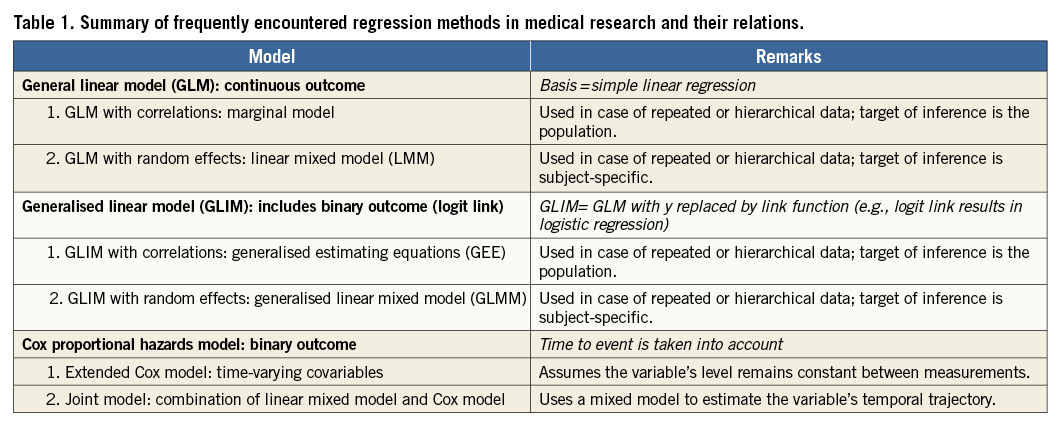
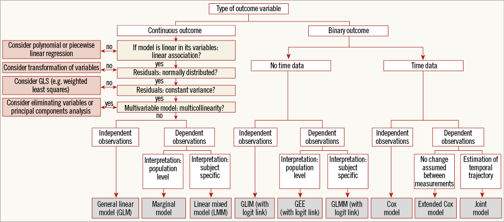
Figure 1. Flow chart.
In linear regression, the dependent variable (y, vertical axis) is continuous, such as for example percent coronary stenosis (for an explanation of types of variables, please see Hoeks et al1). The independent variable (x, horizontal axis) may be binary or continuous, cholesterol level being an example of the latter. When x and y have a linear relation, linear regression can be used to determine the optimal straight line through the sample data points2. In the above-mentioned regression equation, α is the intercept of this line (the value of y when x=0), while β represents the slope and is called the regression coefficient. Specifically, β denotes the number of units of change in y associated with one unit of change in x. Calculation of the linear regression line involves numerous equations. Apart from the aforementioned intercept and regression coefficient, the calculation results in a test of the hypothesis that x and y have a linear relation2. A relation between two biological variables will never be captured perfectly with one line. Therefore, deviations from the line are accepted and represented by the error terms (ε) in the equation: y=α+βx+ε. The error is the difference between the observed value and the regression line we would draw for the total source population. In practice, since we do not have data available on the total source population, we cannot compute this error. The residual is the difference between the observed value and the regression line in the sample. Thus, a residual is an observable estimate of the unobservable error. On the other hand, linear regression determines how much of the total variability in the dependent variable can actually be accounted for by the independent variable. Specifically, this is defined by the coefficient of determination (R2) which is calculated. In univariate models, R2 is the square of Pearson’s correlation coefficient between the independent variable and dependent variable.
Multiple independent (or predictor) variables can simultaneously be tested for their effect on the continuous dependent variable. This is referred to as the “general linear model” (GLM), or multiple linear regression. Computer output will present a table that includes the partial regression coefficients and p-values for each predictor variable2.
An elaborate explanation of linear regression, including its practical applications and example syntax, was recently given by De Ridder et al3.
GLM: ASSUMPTIONS
Several assumptions should be taken into account when considering the use of the GLM4, and, if one or more of these assumptions is violated, the inferences made by the model may no longer be valid (Table 2):

1. The relation between the predictor variables and the outcome variable should be linear.
2. The residuals should be normally distributed with a mean equal to zero.
3. The residuals should have a constant variance.
4. In multivariable models, no multicollinearity should be present.
5. The residuals (for simplicity, we will state “observations” instead of “residuals” in this case) should be independent of each other, i.e., no autocorrelation should be present.
Checking assumptions is further explained by De Ridder et al3. There are several ways to adapt or extend the model in order to deal with violations of assumptions (Table 2, Figure 1). In the following paragraphs, we describe these adaptations and extensions, with the above-described assumptions serving as the outset.
GLM: ADAPTATIONS AND EXTENSIONS
1. GLM FOR ESTIMATING NON-LINEAR RELATIONSHIPS: POLYNOMIAL AND PIECEWISE LINEAR REGRESSION
When the relation between the predictor variables and the outcome variable is not linear, the predictor variables may be transformed in order to draw a curved line through the data points. For example, use of polynomial linear regression models may be considered. Such models contain higher order terms of the independent variable, such as x2 and x3. Including x2 will produce a U-shaped curve (note that, from a statistical point of view, models containing such higher order terms are still called linear if linear in their parameters). Other types of non-linearity may also be modelled, e.g., by using x1*x2, log(x), or ex.
In some cases, the overall relation between the predictor variables and the outcome variable is not linear, but there clearly seem to be multiple different linear relationships in the data, with sudden changes in slope along the x-axis. In such cases, several linear regression models may be constructed for separate ranges of the independent variable, which are connected to each other. This is termed piecewise or segmented linear regression. The points of separation in piecewise regression are called knots. To force the lines to join at the knots, so-called linear spline regression can be applied. An overview of piecewise linear regression has been given in the past by Vieth5.
2. GLM USING TRANSFORMED VARIABLES
When residuals are not distributed normally, the x and/or y variables may be transformed to obtain a normal distribution. This may, for example, be done by using the square root or a logarithmic transformation. After the model is fitted using the transformed variables, the predicted values may be transformed back into the original units using the inverse of the transformation applied.
3. GLM WITH WEIGHTED LEAST SQUARES
The GLM assumes that the variance of the residuals is constant, or in other words that information on y is equally precise over all values of x. This is called homoscedasticity. When, on the other hand, heteroscedasticity is present, the so-called “weighted least squares” (WLS) approach may be used. This is a special case of “generalised least squares” (GLS), which is described in section 5.1 of this paper. WLS incorporates weights, associated with each data point, into the model. Less weight is given to the less precise measurements and more weight to more precise measurements when estimating the unknown parameters in the model. Using weights that are inversely proportional to the variance at each level of the independent variables yields the most precise parameter estimates possible6. WLS regression is further explained by Strutz7. Alternatively, “feasible GLS” (FGLS) may be applied. This approach does not assume a particular structure of heteroscedasticity.
4. GLM: DEALING WITH MULTICOLLINEARITY
Multicollinearity occurs when two or more independent variables in a multivariable regression model are highly correlated. Consequently, the individual coefficient estimates may become unreliable. Multicollinearity may be detected by examining the correlation matrix of the independent variables, the variance inflation factor (VIF; an index which measures how much the variance of an estimated regression coefficient is increased because of multicollinearity), or so-called “eigenvalues”. Remedial measures depend on the research question at hand and include, for example, elimination of some independent variables from the model or performing principal components analysis. Further reading on this topic has been provided by Belsley et al8.
5. GLM: DEALING WITH DEPENDENT OBSERVATIONS/AUTOCORRELATION
5.1. GLM extended with correlations: marginal model
As stated above, for GLMs the assumption that observations are independent of each other applies (Table 2, column 5). This situation is reflected by the data covariance matrix and the data correlation matrix of the GLM. Here, we will focus on the correlation matrix. The correlation matrix of a GLM displays correlations of 0 between residuals of separate observations from the sample (Figure 2A). Such a framework is called “ordinary least squares” (OLS). However, in medical research, observations are not always independent. Such research settings include nested data (e.g., patients within hospitals and hospitals within countries) or repeated measurements data. In the latter case, for example, cholesterol level could be measured repeatedly over time in each patient. If one were randomly to take two observations of cholesterol from the same patient, they are likely to be more similar in value than two random observations of cholesterol from two different patients9. Observations from two different patients may, for their part, be completely independent.
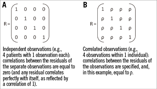
Figure 2. Examples of correlation matrices. A) Independent observations. B) Correlated observations.
Further to this example, since the residuals within one patient are correlated, they need to be modelled. For this purpose, the GLM may be extended by estimating parameters that capture these correlations. This extended GLM is called a marginal model (Table 1, Figure 1)9. The regression line of the marginal model is the same as that of the GLM (y=α+βx+ε). However, the correlation matrix of the marginal model is adapted in such a way that it reflects the pattern of the dependencies between the residuals (Figure 2B). In other words, the OLS framework is extended to a GLS framework. In this framework, the correlations between the residuals within individuals may be specified: they may be set to be equal, but they may also be set to take other patterns. For example, measurements closer in time can have higher correlations than those further away. A number of patterns is readily available in most statistical software packages, such as compound symmetry, auto-regressive patterns, and FGLS (sometimes termed “unstructured”). Of note, correlation matrices still assume that the residuals across different individuals are independent of each other, i.e., that their correlation is zero.
5.2. GLM extended with random effects: linear mixed model (LMM)
Just like marginal models, linear mixed models account for the correlation among the residuals in data with dependent observations (Table 1, Figure 1). However, they use a different approach. They extend the GLM with so-called random effects9-11. We have seen that, for the GLM, the regression line is written as y=α+βx+ε. Here, α and β are so-called fixed regression coefficients, which may be interpreted as population-average effects. The term “mixed” implies that, next to the conventional fixed effects, random effects are incorporated into linear mixed models. These are subject-specific: thus, while fixed effects are constant across individuals, random effects vary between individuals. The linear mixed model may consequently be written as: yi=α+ai+(β+bi)xi+ε, where ai and bi are random effects for subject i (ai=random intercept and bi=random slope). By adding these subject-specific coefficients, linear mixed models account for the fact that measurements within each individual are likely to be more similar. Linear mixed models provide many possibilities. For example, they can accommodate multiple hierarchical levels, like repeated measurements on patients clustered within hospitals.
The choice between a marginal model and a linear mixed model is based on the necessities arising from the data structure, as well as on the interpretation that is preferred. In marginal models, the target of inference is the population, and thus population-averaged coefficients are obtained (while taking into account the dependence of the residuals). In linear mixed models, the target of inference is subject-specific, and thus more precise subject effects may be estimated. An illustrative example is provided by P.D. Allison12: “If you are a doctor and you want an estimate of how much a statin drug will lower your patient’s odds of getting a heart attack, the subject-specific coefficient is the clear choice. On the other hand, if you are a state health official and you want to know how the number of people who die of heart attacks would change if everyone in the at-risk population took the statin drug, you would probably want to use the population-averaged coefficients.”
Binary outcome: generalised linear model (GLIM) and its extensions
GLIM: ADDING A LINK FUNCTION TO GLM
Until now, we have discussed methods to model a continuous outcome. If the outcome is not continuous (but, for example, binary, such as death or myocardial infarction), we need alternative methods. GLIMs (Table 1, Figure 1) generalise the linear modelling framework to outcomes whose residuals are not normally distributed. This is based on the following. A GLIM is made up of a linear predictor, a link function and a variance function (latter not discussed here). The linear predictor resembles the linear regression model and can be defined as: η=α+βx. The link function g(E[y]) is a function of the mean, E[y], (i.e., the expected mean value of y), which is linear in its parameters. In other words, it is a function of the dependent variable which yields a linear function of the independent variables13. Thus, this function describes how the mean depends on the linear predictor: g(E[y])=η. In medical research, GLIMs are most commonly used to model binary data. In that case, the link function is:
![]()
This is called the “logit link”, and the GLIM herewith becomes a logistic regression model:
![]()
where E[y]/(1–E[y]) is the odds of the outcome13. Accordingly, the odds of the outcome can be expressed as eα+βx.
It should be noted that the GLM is a particular case of a GLIM, in which g(E[y])=E[y], since the dependent variable, by definition, is linear in its parameters. This simply leads to E[y]=α+βx (the regression equation previously described). Other link functions are also available, for example the log link is used to model count data which are expected to follow a Poisson distribution (“Poisson regression”). The choice of a particular link function depends on the distribution one wants to choose for the outcome variable.
GLIM EXTENDED WITH CORRELATIONS: GENERALISED ESTIMATING EQUATIONS (GEE)
In parallel to the above description of GLMs with correlations, GLIMs may also be extended by specifying parameters that capture correlations. This combination is called generalised estimating equations (GEE) (Table 1, Figure 1)9,14. When a binary outcome is examined, which necessitates a logistic regression, and repeated measurements of the predictor are performed, then GEE may be used.
GLIM EXTENDED WITH RANDOM EFFECTS: GENERALISED LINEAR MIXED MODEL (GLMM)
Generalised linear mixed models (GLMMs) are GLIMs that are extended with random effects (Table 1, Figure1)15,16. Depending on the interpretation that is preferred (see “linear mixed model”), these models may serve as an alternative when a binary outcome is examined and repeated measurements of the predictor are performed.
Binary outcome taking time into account: Cox proportional hazards model
COX MODEL: BASIC PRINCIPLE
As described above, logistic regression, which is a particular case of a GLIM, may be used to model binary outcomes (for example, death or myocardial infarction). However, logistic regression does not take into consideration the time that passes between the patient’s entry into a study and the occurrence of the outcome. To take time into account, an alternative technique may be used –Cox regression (Table 1, Figure 1)17. A so-called Cox proportional hazards model, or in brief Cox model, is a statistical technique that explores the relationship between several explanatory variables and the time to occurrence of the outcome18. Herewith, it allows us to estimate the hazard (or instantaneous risk) of the outcome for individuals, given their characteristics. It also allows patients to be “censored”, for example at the moment they are lost to follow-up.
The equation of the Cox model is the following:
![]()
Here, ![]() is a function of hazard ratio (or relative risk), α is the coefficient of the constant, and β the coefficient of an independent variable included in the model. An important assumption of the Cox model is the “proportional hazards” assumption17, meaning that the risk ratio of two subjects must remain constant over time (the so-called “log(-log) survival curves” should be parallel and should not intersect). This requires that variables in the model should not interact with time. If this is not the case, an appropriate modification should be used, such as stratification on the variable for which the assumption was violated17.
is a function of hazard ratio (or relative risk), α is the coefficient of the constant, and β the coefficient of an independent variable included in the model. An important assumption of the Cox model is the “proportional hazards” assumption17, meaning that the risk ratio of two subjects must remain constant over time (the so-called “log(-log) survival curves” should be parallel and should not intersect). This requires that variables in the model should not interact with time. If this is not the case, an appropriate modification should be used, such as stratification on the variable for which the assumption was violated17.
EXTENDED COX MODEL
Independent variables in Cox regression may be continuous or binary. Since time is taken into account in Cox regression, the value of a predictor variable does not necessarily need to be fixed from baseline to the end of the study; it may also be allowed to change during follow-up17. Using this possibility may be appropriate when repeated measurements (of, for example, cholesterol level) are performed in each patient, and when the association of this series of repeated measurements is examined with one outcome event (for example, death or myocardial infarction), which occurs after the series of measurements has been performed (Table 1, Figure 1). It should be noted that, when using this type of “time-dependent” variable in a Cox model, a patient reaches an outcome only once. Conversely, in a GLIM (or specifically a logistic regression model) extended with correlations, the outcome variable is assessed concomitantly to the independent variable, i.e., repeatedly. Consequently, the outcome variable is allowed to change multiple times during follow-up (for example, in heart transplant recipients, when the outcome of interest is allograft rejection, this outcome may occur, then abate after treatment, and subsequently re-occur).
Basically, in an extended Cox model, the complete follow-up time for each patient is divided into different time windows, and for each time window a separate Cox analysis is carried out using the specific value of the time-dependent variable. Subsequently, a weighted average of all the time window-specific results is calculated and presented as one relative risk19.
COX MODEL COMBINED WITH MIXED MODEL: JOINT MODEL
The extended Cox model carries limitations, in particular when repeated measurements of continuous variables (such as cholesterol, blood pressure, etc.) are examined20. One such limitation is that the model assumes that, from one measurement to the next, the variable remains constant, and that subsequently a sudden change in the levels occurs on the day the next measurement is performed. However, in reality, variables (such as cholesterol or blood pressure) may change continuously over time. A relatively novel approach that overcomes several limitations of the extended Cox model and that has gained attention recently is the so-called joint model (Table 1, Figure 1). The basic intuitive idea behind joint models is that they combine the Cox model with a mixed model20. Herewith, these models estimate the evolution of the variable over time for each individual patient (mixed model), and relate this temporal profile to the outcome (Cox model). Thus, joint models may be used to examine the association between the detailed time course of a continuous variable with a binary outcome.
Conclusion
When aiming to investigate the association between predictor and outcome variables by using regression analysis, care should be taken to apply the appropriate method. The method of choice should agree with the nature of the data (including the type of outcome variable and the presence of dependent observations) as well as the nature of the research question (including target of inference). Furthermore, assumptions required by the method of choice should be met by the data. The simplified flow chart that summarises some of these aspects (Figure 1) may aid in choosing an appropriate approach. Using the right method will ensure that the analysis will lead to a correct answer to the research question that is being investigated.
Conflict of interest statement
The authors have no conflicts of interest to declare.