Introduction
The statistical method used for analysing a clinical outcome is mainly determined by the measurement type of the outcome variable. For example, a dichotomous outcome such as “restenosis after 6 months” or “successful intervention” is analysed with a method that is different from that which would be used to analyse a continuous outcome such as “minimum lumen diameter” or “percentage of restenosis”. In this paper we will focus on the situation in which there is a continuous outcome.
An appropriate method to analyse a continuous outcome is (under certain conditions) linear regression analysis. This method enables using all information embedded in the observed values of the outcome and investigating the relationships between this outcome and other continuous and categorical variables, the so-called explanatory variables. The effects of these explanatory variables might be studied one at a time (simple regression) or simultaneously (multiple regression). The inclusion of several explanatory variables, as in a multiple regression, can also be used to correct for confounders (variables related to both the outcome and the explanatory variable of interest, e.g., treatment) in order to avoid biased results. When other variables explain a considerable part of the variation in the outcome, the effect of the explanatory variable of interest might only be detectable after adjustment for these covariates. Besides this, regression analysis can be used to develop a prediction model for the outcome.
In this paper we will discuss some aspects of linear regression analysis. A more detailed explanation and instructions on how to apply the methods using SPSS or SAS are given in the Online Appendix. Since terminology concerning linear regression (and statistics in general) used in the literature, handbooks and statistical software is not consistent, an overview of some terms can also be found in the Online Appendix.
Description of example data
The data used in the examples in this paper come from the LEADERS study1. In this study 1,700 patients with one or more coronary artery stenoses >50% in a native coronary artery or a saphenous bypass graft were randomised to treatment with either biolimus-eluting stents (BES) with biodegradable polymer or sirolimus-eluting stents (SES) with durable polymer. One fourth of the study group was randomly assigned (1:3 allocation) to undergo follow-up angiography at nine months. The LEADERS study was designed to investigate non-inferiority of BES compared to SES regarding the primary composite endpoint of cardiac death, myocardial infarction and clinically indicated target vessel revascularisation within nine months.
In this paper we will focus on a continuous outcome, namely the minimum lumen diameter (MLD) in the stented segment, measured at the follow-up visit nine months after the intervention. A protective effect of high-density lipoprotein cholesterol (HDL) on coronary heart disease has already been established since the late 1970s2. We will deal with investigating the relation between the explanatory variable HDL, measured at baseline, and minimum lumen diameter (MLD), measured after nine months. We selected patients with both nine-month follow-up measurement of MLD and baseline HDL available, and will only use the measurement on one stent for these patients (n=243). The genetic characteristic (variable GENTYPE), used in example models in the Online Appendix, does not reflect real data, but is generated to provide a useful example.
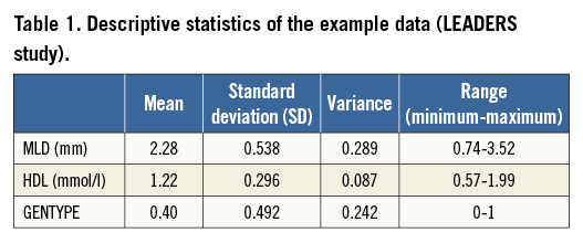
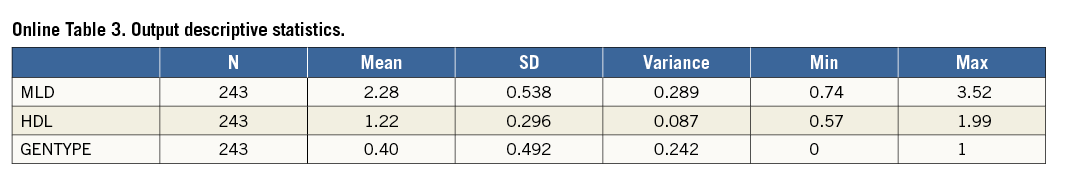
Descriptive statistics of the data are given in Table 1.
Research questions related to linear regression
When considering the relation between one continuous explanatory variable (HDL) and the outcome (MLD), some questions which could be addressed include the following:
– If patient A has a higher HDL than patient B, can we expect the MLD of patient A to be higher than the MLD of patient B?
– If so, how much higher is (the expected) MLD if HDL is 1 mmol/l higher?
– If we know the HDL of a patient, which value of MLD can we expect?
– How wide is the confidence interval around this expected MLD?
– In case there is a relationship between HDL and MLD, is this relationship the same in different genetic subgroups?
– A patient’s age may influence both HDL and MLD. What is the relation between HDL and MLD if adjusted for the influence of age?
Linear regression can also be used to find a model to predict the outcome variable. Questions might be:
– Which baseline characteristics of a patient can be used to predict MLD?
– How accurate is this prediction of MLD?
– Will the accuracy of the prediction of MLD significantly improve if another variable (for example a lab measurement not commonly available) is added to the model?
– Which percentage of the variability in the outcome variable MLD is explained by the model?
When to apply linear regression
One of the crucial conditions in applying linear regression analysis is that a continuous outcome is involved and the effect of one or more explanatory variables on this outcome is of interest. Regression should not be confused with correlation, which focuses on the strength of the relation between two continuous variables without defining one of them as outcome, and without estimating effects. In principle, the explanatory variable(s) can be of different types: continuous, dichotomous (only two possible values), or categorical with more than two discrete values. However, if there is only one explanatory variable and this variable is not continuous, other analyses might be preferred, i.e., for a dichotomous explanatory variable, a two-sample t-test, and, for a categorical explanatory variable with more than two categories, a one-way analysis of variance.
Prior to applying a linear regression model, it is important to create a scatter plot of the continuous explanatory variable (often indicated as the X variable in the relation) HDL and the outcome variable (Y variable) MLD. This plot enables checking the (X, Y) pairs and gives information about the shape and direction of the relationship. Furthermore, three required assumptions can be checked:
1. The straight line relationship between HDL (X) and the expected values of MLD (Y).
2. For each value of HDL, the values of MLD should have a normal distribution around the expected value.
3. The variability of this normal distribution should be the same for all values of HDL.
Figure 1 shows scatter plots of six hypothetical relations. For the data points in Figure 1A, Figure 1B and Figure 1C the assumptions hold. The presence of a significant relation still needs to be tested. In Figure 1D the relationship is not a straight line. In Figure 1E the variability of Y is not independent of X, but clearly increasing with increasing X. Also in Figure 1F the spread of Y values is not constant: there seems to be a lower threshold for values of Y (e.g., value 0).
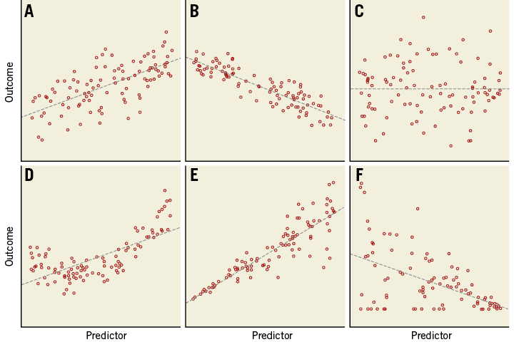
Figure 1. Scatter plots of six relations. Dashed lines are the fitted linear regression lines. A) Linear, positive relationship; B) linear, negative relationship; C) linear, neutral or no relationship; D) non-linear relationship, the regression line does not fit to these data; E) linear, but increasing variance with increasing value of the predictor; F) negative relationship, but decreasing variance and over-representation of outcome value 0.
When one of these assumptions is not fulfilled, some adaptation might provide an appropriate situation that allows linear regression, e.g., applying a transformation on the X or Y values.
A fourth assumption for applying linear regression is the independency of the observations. For example, if patients have more than one stent with a measured MLD value, observations in the same patient are related. For such data, applying a linear mixed model (repeated measurements analysis) would probably be suitable.
Results from a simple regression analysis
For simple regression (one explanatory variable), fitting the model means that the “best fitting” straight line through the scatter plot of outcome variable versus explanatory variable is calculated (Figure 2, Table 2). The output of a regression analysis, for example in SPSS or SAS, will give the estimated value of the intercept, i.e., the expected MLD at HDL=0, and the slope of this line. These determine the regression equation which allows calculation of expected values for the outcome, given a value of the explanatory variable, e.g., Expected (MLD)=1.978+0.250*HDL. In this specific example, the estimate value for the intercept (1.978) is only of limited value since zero is not a realistic value for HDL. The slope of 0.250 indicates that when HDL increases by one unit, the expected MLD increases by 0.250.
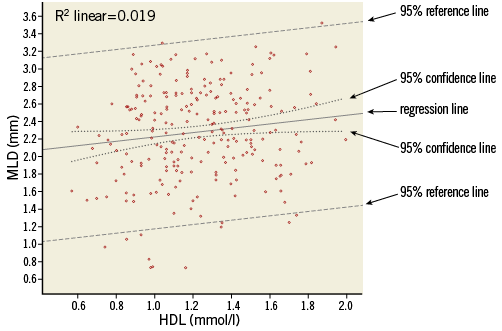
Figure 2. Scatter plot of MLD versus HDL, with data points, regression line, 95% confidence lines (dotted lines close to the regression line) and 95% reference lines (dashed lines).
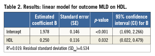
Because the intercept and slope of the regression line are estimated using a limited number of subjects (in this example n=243), we cannot be 100% sure that we have found the correct regression equation that will apply for the complete population from which the study group is sampled. Therefore, for both estimated coefficients, the standard error is given. This standard error of the coefficient is, just like a standard error of the mean, used to determine a confidence interval and to provide the significance of testing the null hypothesis: H0: regression coefficient=0. A 95% confidence interval not including zero will correspond with a significance (p-value) below 0.05. If such results are obtained for the slope, this indicates a significant relationship (on the usual level of significance α=0.05) between explanatory and outcome variable.
It should be stressed that this statistically significant relation does not necessarily mean that there is a clinically relevant association3. Whether, for example, this finding justifies further HDL level monitoring of a patient post intervention should be based on clinical knowledge.
The regression equation does not fix the relation between X and Y completely. Figure 2 shows that, for each value of HDL, the observed data points scatter around the expected value of MLD on the regression line, and so will data points of other (new) patients. The amount of variability of MLD, given a value of HDL, can be described by the residual standard deviation (SDres), which for this relation has a value of 0.534. This residual standard deviation (i.e., deviation after model fitting) will be smaller than the “crude” standard deviation, to a greater or lesser extent, depending on the relation. In Figure 2, lines at distances 1.96 times the residual standard deviation from the regression line are drawn. These reference lines determine the 95% reference or prediction intervals for MLD, conditioned on HDL. Roughly 95% of the data points will lie between the two lines. The reference lines should not be confused with the 95% confidence lines, which indicate the precision of the regression line (95% confidence intervals for the expected values).
While HDL is a significant predictor for MLD, we could ask whether HDL is also an “important” predictor for MLD. The answer is - “It is not very important”. The R2, square of the correlation coefficient R, indicates how much of the variability in MLD values is explained by HDL. Since this is only 1.9%, the other 98.1% might possibly be explained by other patient characteristics. This weak relation between the variables can be seen in the wide spread of data points around the regression line and is also reflected in the small difference between the original (unadjusted) standard deviation of MLD (=0.538, Table 1) and the residual standard deviation of 0.534 (Table 2).
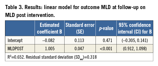
A much stronger relationship is found if MLD at nine-month follow-up is related to MLD measured immediately after the intervention (Figure 3, Table 3). Here, the R2 is 0.632: therefore, 63.2% of the variability of MLD at follow-up is explained by the previously measured MLD. The slope is highly significant and its estimated value of 1.005 indicates that every extra millimetre of MLD post intervention gives an extra millimetre at follow-up.
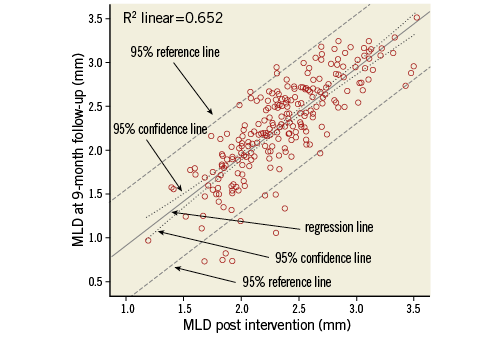
Figure 3. Scatter plot of MLD at follow-up versus MLD post intervention, with regression line, 95% confidence lines (dotted lines close to the regression line) and 95% reference lines (dashed lines).
Extending the model
A simple regression model can be extended with other explanatory variables (multiple regression analysis), either continuous or categorical (note that adding a categorical variable with more than two categories requires the use of dummy variables; Online Appendix).
The interpretation of the regression coefficients in a multiple regression model is somewhat different from in a simple regression model. Regression coefficients in a multiple regression model give the estimated change in the outcome variable for one unit change of the explanatory variable, keeping all other explanatory variables fixed.
The effect of an explanatory variable on the outcome might depend on the value of other variables. For example, HDL may have a strong effect on MLD in patients with a certain genetic characteristic, while in other patients this effect is less strong or even not present, or the effect might increase or decrease with increasing age. The size of a treatment effect can vary between patients with different characteristics. Such interactions can be investigated by testing the significance of interaction terms (Online Appendix).
Obviously, an interaction should only be investigated if this is motivated by a hypothesis.
How to report a linear regression
When the results of a linear regression are described, it is obviously necessary to report what is the outcome variable in the model and which are the explanatory variables. For a multiple regression model the reasoning and motivation as to which independent variables were included should be explained. Was this fixed beforehand? Was the goal to estimate the effect of a specific variable, and were the other variables added to adjust for confounding? Was the objective to obtain a model with a high percentage of explained variance? Was inclusion of variables guided by their significance? Were interaction terms considered?
The resulting model is best described by presenting a table with the estimated regression coefficients, their standard error or (95%) confidence interval and, optionally, the p-value. To enable readers to calculate predictions, the estimated value for the intercept should also be reported, next to the regression coefficients of all variables in the model, including the adjusting variables. If the focus is on one or some specific explanatory variables and the other variables were only needed for adjustment, results for these adjusting variables may be omitted. However, it should be clearly stated that these variables were included, for instance with an accompanying footnote in the table. The meaning of an estimated effect can be explained in words, such as “for patients of the same age and gender, an increase in systolic blood pressure of 10 mmHg gives a decrease in MLD of 3.6 mm”.
If the purpose of the model is to give predictions for new subjects, the R2 should be reported, as well as information about the width of prediction intervals.
Conclusions and recommendations
Linear regression is the most suitable method to analyse how explanatory variables can explain or predict a continuous outcome variable. It allows effect estimation and testing the significance of these effects. Output from a regression analysis also shows the percentage of variability of the outcome variable that is explained by the explanatory variable(s).
Visualising the data in a scatter plot(s) should be the first step when considering a linear regression, to check whether the assumptions are fulfilled.
The variables and interactions used in a model should be specified initially, based on research questions. Inclusion of covariates in a final model can be guided by the data, but should be based on pre-specified criteria, for example the significance of the covariate <0.10, or a change in the estimated effect of the main explanatory variable of more than 10%.
In this paper we have attempted to provide some practical information about using linear regression for the explanation or prediction of a clinical outcome variable, based on one or more explanatory variables such as lab measurements, patient characteristics, treatment characteristics, etc. For more detailed material on the subject as well as problem solving exercises, we recommend further reading4-7.
Conflict of interest statement
The authors have no conflicts of interest to declare.
Online Appendix. Instructions and detailed explanation
INTRODUCTION
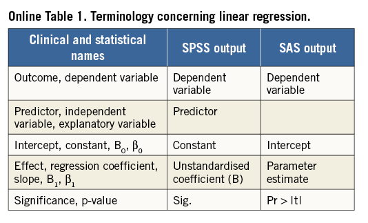
This appendix contains instructions on how to apply the methods discussed in the paper using (IBM) SPSS or SAS. For SPSS, instructions for using the menu as well as the command syntax are given. All variable and dataset names for the specific variables, corresponding to the examples, are printed in bold. The output shown is SPSS output. Paragraphs in this appendix correspond to paragraphs in the paper. An overview of some terms concerning linear regression is given in Online Table 1.
DESCRIPTION OF EXAMPLE DATA
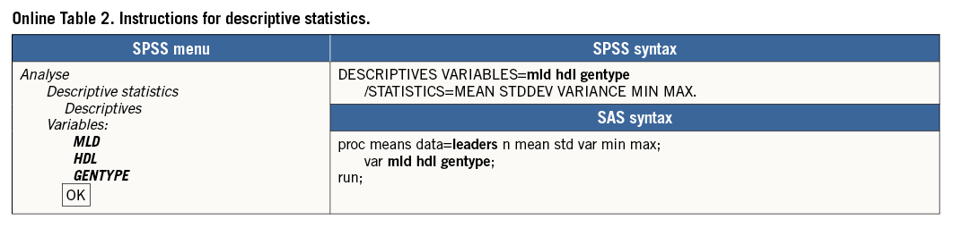
Online Table 2 shows how descriptive statistics can be obtained, using the SPSS menu, SPSS syntax or SAS syntax. The results are shown in Online Table 3.
WHEN TO APPLY LINEAR REGRESSION
Next to the assumptions mentioned in the paper, a more technical assumption is that the explanatory variable is measured without error. Measurement error, if any, should only be present in the dependent variable.
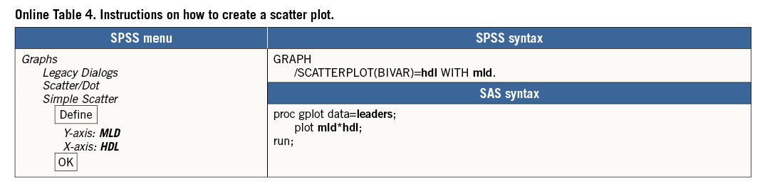
A very important first step is to visualise the relation between HDL and MLD with a scatter plot, HDL and MLD both being continuous variables. To do this, we need to decide which variable is the dependent variable and which the explanatory variable. A “proven” causal relationship is not necessary to make this distinction; however, in our example it is obvious to make HDL the explanatory variable. Therefore, in the scatter plot the observed values of HDL determine the horizontal location of the dots (X axis) and the values of MLD, the dependent variable, determine the vertical location (Y axis) (Online Table 4).
In the scatter plot in Online Figure 1, we see 243 dots representing the MLD and HDL values of the patients. Point P represents a patient whose HDL is 1.6 mmol/l and MLD is 2.75 mm.
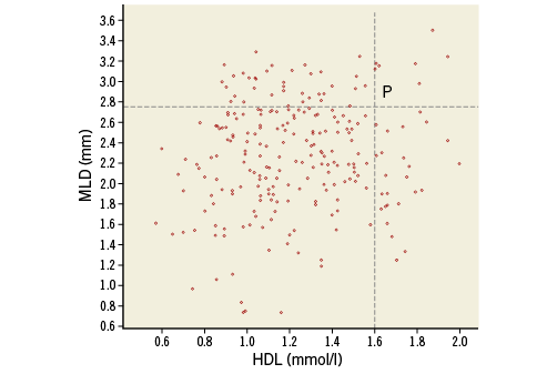
Online Figure 1. Scatter plot of MLD versus HDL.
The scatter plot shows a weak relationship between HDL and MLD. Patients with a higher HDL tend to have a higher MLD. It is certainly not a one-to-one relation (like a mathematical function): a value of HDL is not linked to only one value of MLD. Patients with HDL below 1.0 mmol/l have values of MLD between 0.5 and 3.4 mm, while patients with HDL above 1.5 mmol/l have values of MLD between 1.25 and 3.6 mm.
RESULTS FROM A SIMPLE REGRESSION ANALYSIS
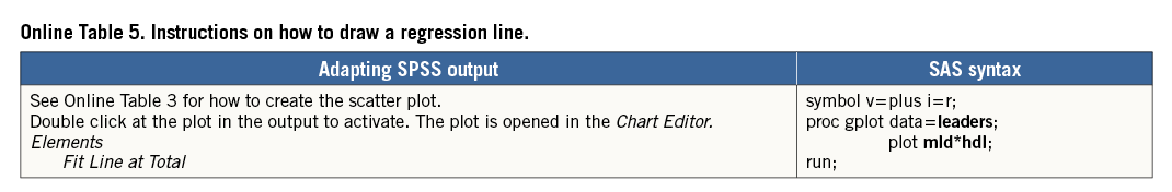
The “best fitting” line through a scatter plot is defined as the line for which the sum of (squared) vertical distances of all observed data points to that line is minimal (Online Table 5, Online Table 6, Online Figure 2).
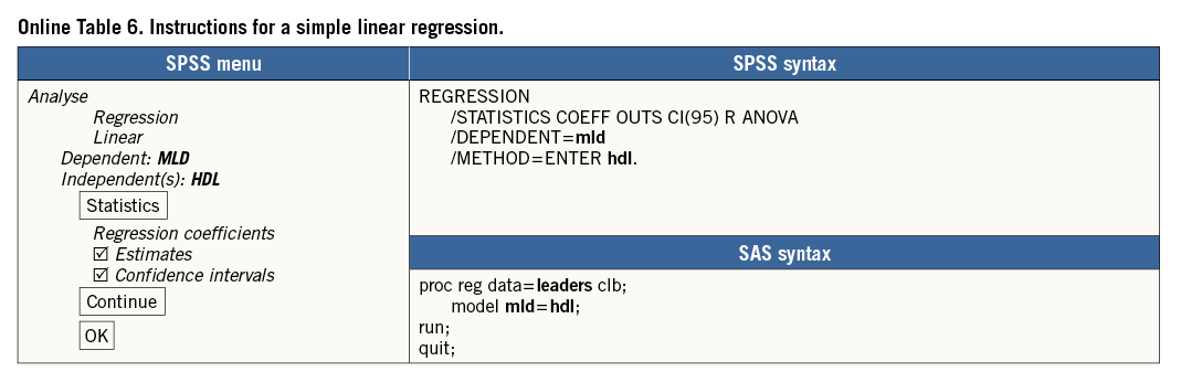
Online Figure 2. Scatter plot with data points and regression line.
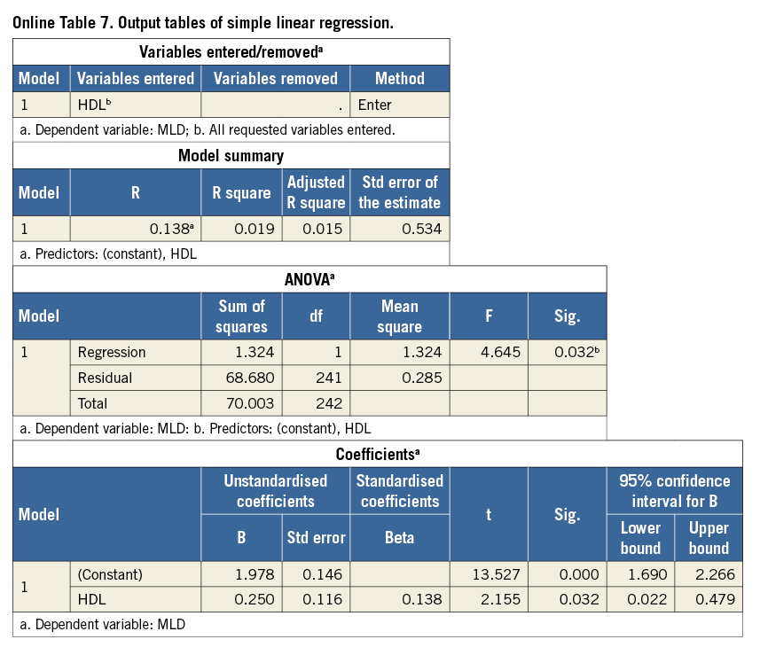
We start focusing on the last table in the output (Online Table 7), the coefficients table. Using the estimated coefficients (Unstandardised coefficients, column B) we can write down the regression equation for the best fitting line. This equation is a mathematical function: each value of HDL is related to one value of the expected MLD, denoted by ![]() (“MLD hat”) or by E(MLD|HDL): expected value of MLD, given a value for HDL:
(“MLD hat”) or by E(MLD|HDL): expected value of MLD, given a value for HDL:
E(MLD|HDL)=1.978+0.250*HDL (1)
The first value in equation (1), 1.978, is the intercept of the regression line: the Y-value of the point of the line when X=0. SPSS uses the name Constant instead of intercept. This indicates that 1.978 is the expected value of MLD when HDL=0, because E(MLD|HDL=0)=1.978+0.250*0=1.978. However, the value 0 is an impossible value for HDL, so this does not reflect a realistic data point. The second value in equation (1), 0.250, is called the regression coefficient or slope. This value has much more practical meaning than the intercept because it indicates how “steeply” the regression line increases with increasing HDL. For instance, the expected value for MLD when HDL=1 is calculated as E(MLD|HDL=1)=1.978+0.250*1=2.228. If HDL increases by 1, the expected value for MLD will increase by the value of this slope, 0.250: E(MLD|HDL=2)= 1.978+0.250*2=2.478.
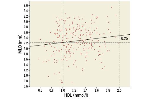
Using the regression equation, we can calculate for each value of HDL the expected (sometimes called predicted) value of MLD. This regression line is plotted in Online Figure 2. The increase of 0.250 in MLD when HDL changes from 1.0 to 2.0 is indicated.
Because the intercept and slope of the regression line are estimated using a limited number of data points (in this example n=243), we cannot be 100% sure that we have found the correct regression equation that will apply for the complete population. For both estimated values, SPSS gives the standard error (Std error, Online Table 7, Coefficients). What is important is whether we can (or cannot) be certain that there is a real relation between HDL and MLD, i.e., that the slope is different from zero. A zero slope would mean that the value of HDL is not at all predictive for the value of MLD. In the column Sig., still in the Coefficients table, we can find the p-value for the (two-sided) test of the null hypothesis: H0: regression coefficient=0. For the regression coefficient of HDL in this model p=0.032. Applying the usual significance level α=0.05, we reject this null hypothesis, indicating a significant relationship between HDL and MLD. Also, the 95% confidence interval (CI) (columns at the right: 95% CI=[0.022 to 0.479]) indicates that zero is a very unlikely value for the slope, because zero is not included in this CI. This is another way to show that there appears to be a significant relation between HDL and MLD (for the intercept, p-value and CI are also given, but these have limited value in this particular example).
As noted before, the regression equation (1) does not fix the relation between HDL and MLD completely. For a given value of HDL, e.g., HDL=1.5, the observed data points scatter around the expected value of MLD of 2.353 and so will data points of other (new) patients with HDL=1.5. The amount of variability, given a value of HDL, can be described by the residual standard deviation (named Std. Error of the Estimate in the SPSS output, Online Table 7, Model Summary). In this example the residual standard deviation has a value of 0.534. This value can be compared to the ordinary standard deviation of the outcome MLD, which describes the variation of MLD values around its mean. We saw (Online Table 3) that this standard deviation was 0.538, so in this example the residual standard deviation is only slightly smaller. In Online Figure 3, lines at a distance 1.96 times the residual standard deviation from the regression line are drawn. These lines determine the 95% prediction intervals for MLD, conditioned on HDL. Around the predicted MLD of 2.228 mm for an HDL of 1 mmol/l, the 95% prediction interval is 1.181 to 3.275. Roughly 95% of the data points will lie between the two lines.
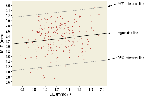
Online Figure 3. Scatter plot with data points, regression line and 95% reference lines.
Now that we know HDL is a significant predictor for MLD, we could ask whether HDL is also an “important” predictor for MLD. The answer is - “It is not very important”. The value of R2 in the table Model Summary (Online Table 7), 0.019, indicates how much of the variability in MLD values is explained by HDL. Since this is only 1.9%, the other 98.1% might possibly be explained by other patient characteristics. This weak relation between the variables can be seen in the wide spread of data points around the regression line and is also reflected in the small difference between original (unadjusted) and residual standard deviation.
EXTENDING THE MODEL
Adding a second continuous explanatory variable is simply done by specifying this in the box Independent(s). A dichotomous explanatory variable can be added in the same way. Most appropriate is to code this variable with values 0 and 1.
If GENTYPE is added to the model of MLD regressed on HDL as a second independent variable, the output shows a table with coefficients as displayed in Online Table 8.
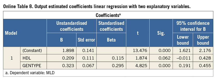
These estimates indicate that a predicted value for MLD using this model is described by:
E(MLD|HDL, GENTYPE)=1.898+0.209*HDL+0.323*GENTYPE (2)
If we consider patients with GENTYPE=0, the third term at the right side of the equation is 0, so it can be disregarded. The resulting equation represents a line with intercept 1.898 and slope 0.209. For patients with GENTYPE=1, the predicted value is just enlarged with value 0.323. Plotting the predicted values gives two parallel regression lines (Online Figure 4).
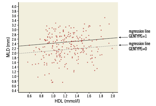
Online Figure 4. Scatter plot with parallel regression lines for the genetic groups (model without interaction). Squares and solid line: GENTYPE=1, Xs and dotted line: GENTYPE 0.
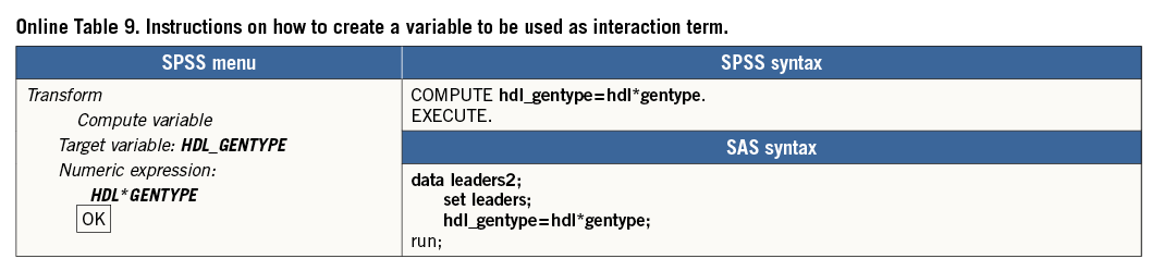
The plot shows clearly that this model assumes that the effect of HDL on MLD does not interact with the effect of GENTYPE on MLD: regardless of the value of GENTYPE, the predicted MLD always increases with 0.209 if HDL increases by one (parallel lines have equal slope). This also holds the other way round: for every value of HDL, the difference in predicted MLD between a patient with GENTYPE=1 and GENTYPE=0 is always 0.323 (the distance between parallel lines is constant). To investigate if this is correct, or if the effects do interact, we could add the interaction term HDL*GENTYPE to the model and check its significance. In SPSS a new variable has to be created indicating this interaction, calculated as the product of variables HDL and GENTYPE. Note that this variable has the value of 0 for all patients with GENTYPE=0 and is just a copy of HDL for all patients with GENTYPE=1 (Online Table 9).
Running the model with independent variables HDL, GENTYPE plus the interaction variable HDL_GENTYPE results in the estimated coefficients presented in Online Table 10.
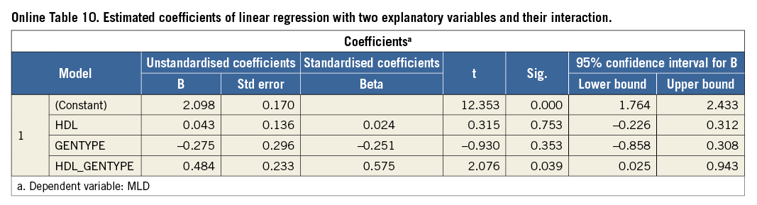
Given values for HDL and GENTYPE, a prediction for MLD is now expressed as:
E(MLD|HDL, GENTYPE)=2.098+0.043*HDL–0.275* GENTYPE +0.484*HDL*GENTYPE (3)
The significance for the interaction term is p=0.039, so below 0.05, indicating that this coefficient is significantly different from zero, and is therefore not negligible (the significance of the main terms HDL and GENTYPE, which are both above 0.05, is of less importance. They should not be removed from the model as long as the interaction term is included).
Substituting in (3) GENTYPE=0 and GENTYPE=1, respectively, results in the following equations to calculate the predicted value of MLD for the two genetic groups:
E(MLD|HDL, GENTYPE=0)=2.098+0.043*HDL (4)
E(MLD|HDL, GENTYPE=1)=1.823+0.527*HDL (5)
These equations clearly show that for GENTYPE=0 MLD is almost unrelated to HDL (slope 0.043), while for GENTYPE=1 the relation is much stronger (slope 0.527). So the relation between HDL and MLD is dependent on the value of GENTYPE (arguing the other way round, we can say that the effect of GENTYPE is not constant, but depends on the value of HDL, e.g., when HDL=1, the predicted difference in MLD between the genetic groups is –0.275+0.484*1=0.211; when HDL=2 this difference is –0.275+0.484*2=0.693).
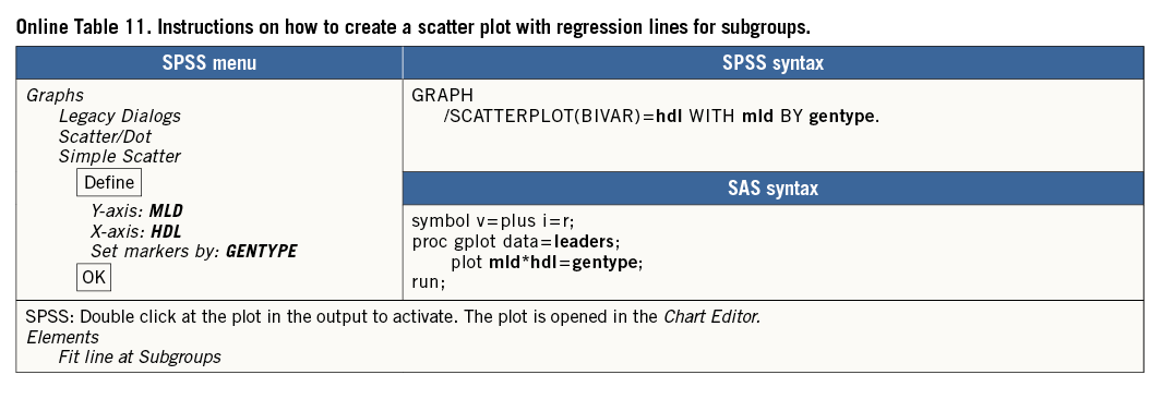
A scatter plot with the two lines for the subgroups, as given in Online Figure 5, can easily be created (Online Table 11).
If we wanted to use a categorical explanatory variable with more than two categories in a linear regression procedure, it would require creation of dummy variables. Alternatively, we could switch to applying the procedure (univariate) general linear model, with categorical variables indicated as fixed factor(s) and continuous variables as covariate(s). However, further discussion about this procedure is beyond the scope of this paper.
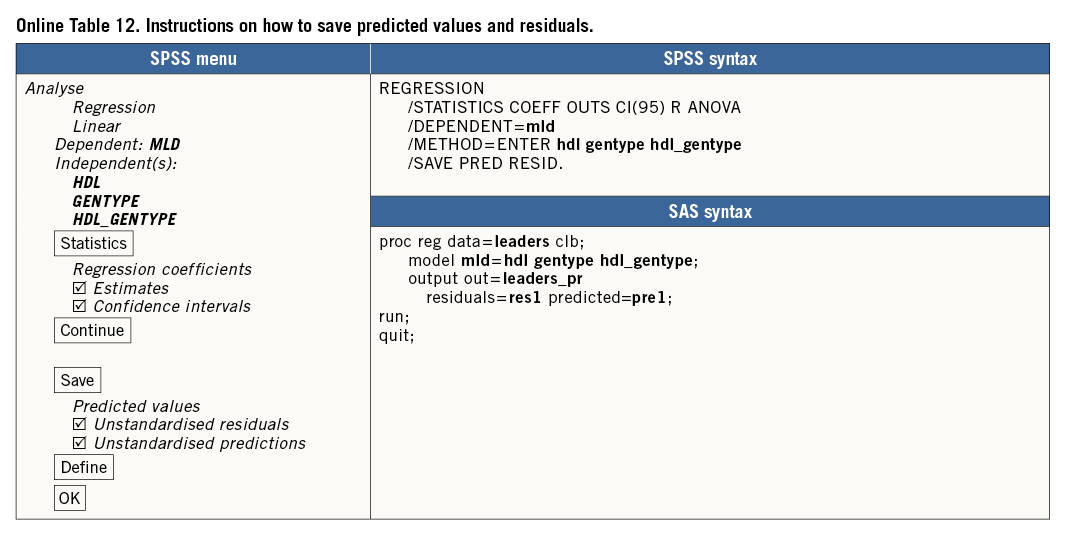
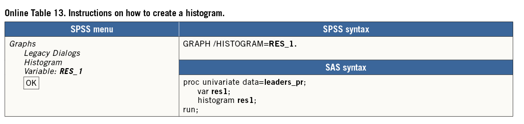
To check the assumptions in a multiple regression model, again, plotting the outcome variable versus each continuous explanatory variable may be useful, if applicable using different symbols for subgroups, as shown in Online Figure 4 and Online Figure 5. Furthermore, the residuals of the regression (observed minus predicted value of the outcome variable) should be plotted versus the different explanatory variables and versus the predicted values. (Online Table 12 shows how to save residuals and predicted values from a linear regression.) The residuals should randomly scatter around 0 for all values of X. A histogram of the residuals should show a bell-shaped (normal) distribution (Online Table 13, Online Figure 6).
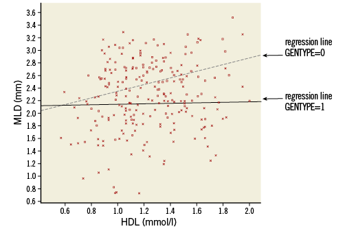
Online Figure 5. Scatter plot with regression lines for the genetic groups (model with interaction). Squares and solid line: GENTYPE=1, Xs and dotted line: GENTYPE=0.
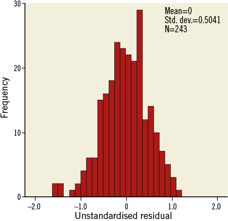
Online Figure 6. Histogram of residuals.