Introduction
In clinical research, we often examine continuous variables such as blood pressure, ejection fraction, laboratory values (e.g., cholesterol), and angiographic variables (e.g., percent stenosis). We may, for example, want to compare these measurements between different patients or between different time points. To compare continuous data, parametric or non-parametric tests of significance may be applied. Which of these tests is appropriate depends on several factors, including the nature of the data to be analysed. These data should meet the assumptions that are required for the particular test. This paper describes parametric methods and the circumstances under which these methods are appropriate. Its aim is to give a general overview, without claiming completeness; hence, exceptions are possible in specific situations.
Basic considerations
DISTRIBUTION OF DATA
When continuous (i.e., interval or ratio) data are organised and graphed as a histogram, they take on a shape referred to as a distribution1. The most common distribution is the normal curve, which is symmetric and has a shape that resembles a bell (Figure 1). However, a distribution may also be skewed, i.e., not symmetric2. For example, a distribution can be positively skewed when most of the measurements occur at the lower end of the distribution.
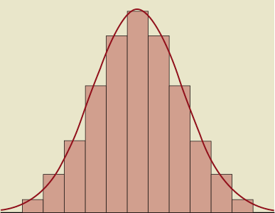
Figure 1. Histogram and normal distribution.
MEAN AND MEDIAN
The arithmetic mean is the sum of all values, divided by the number of values. The median is the value that divides the distribution in half, i.e., if the observations are arranged in increasing order, the median is the middle observation2. Thus, half of the observations are above the median and half are below it. If there is an even number of observations, there is no middle one and the average of the two “middle” ones is taken. To summarise a variable, it is usually recommended that, when a variable follows a normal distribution, the mean and standard deviation (SD) should be reported. When a variable does not follow a normal distribution, the mean may be unrepresentative of the majority of the data2. In that case, the median and range (e.g., 25th and 75th percentile) should be reported instead. Furthermore, since the mean is very sensitive to outliers, to which the median is more robust, it is preferable to report the median and range when the distribution shows extreme cases, despite being expected to be normal.
STATISTICAL SIGNIFICANCE
In short, hypothesis testing is based on the following. The null hypothesis states that there is no difference between the study groups; for example, it states that mean blood pressure is the same in group 1 and group 2, or that blood pressure is the same before receiving medication and after receiving medication. The null hypothesis can be true or false. Statistical tests determine the probability that the null hypothesis is erroneously rejected; this probability is called a p-value (or “alpha level”)1. The smaller the p-value, the stronger is the evidence against the null hypothesis. The cut-off point of the p-value is usually set at 0.05 and is called the significance level. There are numerous statistical tests available; in this paper we focus on two commonly used parametric tests.
Choosing between parametric and non-parametric methods
Parametric methods are appropriate when data are measured on the interval or ratio scale and when they are distributed normally. Normality of the data may be examined by visual examination of histograms, box plots or Q-Q plots and by performing tests of normality such as the Kolmogorov-Smirnov test or the Shapiro-Wilk test3. If the data are not distributed normally, non-parametric statistical methods are appropriate4. Non-parametric methods are also more appropriate when one is dealing with small samples, since in such cases it is often difficult to assess the normality of the distribution of the data5, and the influence of extreme data points on the mean is larger.
Parametric tests are typically more powerful than non-parametric tests, meaning that if a difference between the study groups truly exists, that difference is more likely to be found using the parametric test4. However, because not all data are normally distributed or measured on an interval or ratio scale, in some cases only non-parametric methods can be applied.
Parametric tests
T-TEST
The t-test, also called Student’s t-test, is one of the most commonly used methods in clinical research6. It is a parametric method that is based on the means and SDs or variances of the data4. There are several assumptions for using the t-test: the sample data must be derived from a normally distributed population; for two sample tests, the two populations must have equal variances; and each measurement (or the difference score for dependent data) must be independent of all other measurements1,3. In case the assumption of equal variances is not fulfilled, Welch’s t-test may be used as described elsewhere7.
Several types of t-test exist3,4,6,7. The one-sample t-test is applied when one study group is examined and may be used to compare the group mean to a theoretical mean. The paired t-test is used to estimate whether the means of two related sets of measurements are significantly different from one another. This test is used when measurements are dependent because they are collected a) from the same participant at different times, b) from different sites on the same person at the same time, or c) from cases and their matched controls3. When two study groups are examined and the measurements performed in the groups are independent (which, for example, applies to an [unmatched] control versus experimental group design), an independent two-sample t-test is appropriate.
When a group mean is compared to a theoretical mean (one-sample t-test), the null hypothesis states that the group mean is equal to this theoretical mean. The t-statistic is calculated as the difference between the group mean and the hypothesised value of the group mean, divided by the standard error (SE) of the mean (Figure 2, equation 1)6. The SE may be substituted by the SD divided by the square root of the number of subjects (equation 1). For example, suppose that in a certain medical centre mean systolic blood pressure in patients treated for stable angina pectoris is 124 mmHg. We want to test whether the mean systolic blood pressure in patients with stable angina in our own centre is different from our hypothesised value of 124 mmHg. Our study population consists of 100 patients. Suppose that we measure a mean systolic blood pressure of 132 mmHg with an SD of 23 mmHg in our study population. In this case, t is equal to (132-124)/(23/√100)=3.48. The accompanying p-value, as derived from a table of critical values for t, is <0.001. Thus, we conclude that the null hypothesis (“mean systolic blood pressure in our study population is equal to 124 mmHg”) may be rejected at the 0.05 level (and in this case even at the 0.001 level). These results can also be easily obtained from statistical software programmes.
To compare the means of two dependent sets of measurements, such as repeated measurements performed on patients from one single group, a paired t-test is used. Suppose we want to test in our study population of 100 patients with stable angina whether the mean systolic blood pressure before receiving certain medication is the same as that after receiving the medication. In this case, t is calculated as the mean difference between the measurements at the two time points, divided by the SE of this difference (Figure 2, equation 2)6. Again, the SE may be substituted by the SD (in this case, the SD of the mean difference), divided by the square root of the number of subjects. It should be noted that the SD of the mean difference is not merely a combination of the SDs of the means at the two time points, but is calculated from the total number of mean differences. Suppose that in our data we find a mean difference in systolic blood pressure of 5 mmHg with an SD of 4 mmHg. Consequently, t is equal to 5 / (4/√100)=12.5. Once more, this renders a p-value <0.001.
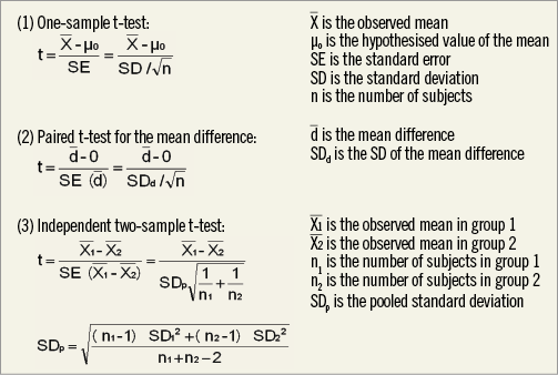
Figure 2. t-test: calculation of t.
To compare the means of two independent sets of measurements (independent two-sample t-test), t is calculated as the difference between the two group means divided by the SE of this difference (Figure 2, equation 3)6. The SE of the difference can be calculated from the pooled SD and the numbers of subjects of both groups, as depicted in equation 3. The pooled SD, for its part, can be calculated from the SDs of each of the groups and the number of subjects of both groups (Figure 2). Suppose we want to investigate whether in our study population of 100 patients with stable angina systolic blood pressure in men is the same as systolic blood pressure in women. Suppose there are 30 women with a mean systolic blood pressure of 134 mmHg, and 70 men with a mean systolic blood pressure of 131 mmHg, and the pooled SD is 24 mmHg. The SE of the difference then equals 24* √(1/30+1/70)=5.2. Thus, t=(134 –131/5.2)=0.58, and the accompanying p-value is >0.5. We conclude that the null hypothesis may not be rejected at the 0.05 level.
ANOVA
When more than two groups are compared using multiple t-tests, the probability of rejecting a true null hypothesis is increased as the number of comparisons made using independent t-tests increases4. Analysis of variance (ANOVA) is the appropriate statistical method to test for differences among three or more groups3. The assumptions for ANOVA are similar to those for the t-test (i.e., normal distribution; equal variances; each measurement independent of all other measurements)3,4,6.
The general theory behind the calculations of ANOVA is based on the following. ANOVA considers the variation in all observations and divides it into: a) the variation between each subject and the subject’s group mean, and b) the variation between each group mean and the grand mean6. If the group means are quite different from one another, considerable variation will occur between them and the grand mean, compared with the variation within each group. If the group means are not very different, the variation between them and the grand mean will not be much more than the variation among the subjects within each group6. The concept of ANOVA can be thought of as an extension of a two-sample t-test but the terminology used is different3. Just as the t-test uses calculation of a t-statistic, ANOVA uses calculation of an F-ratio. This F-ratio is defined as (between-groups variance) / (within-group variance), and indicates whether the variability between the groups is large enough compared to the variability of data within each group to justify the conclusion that two or more of the groups differ3,4,6. If an ANOVA was being used instead of the t-test to compare two groups, it would be found that F=t2 for these data4. After obtaining the F-ratio, it may be compared to the critical F-ratio in order to find the p-value. In our example of patients with stable angina, we would apply ANOVA if, for example, we wanted to test whether systolic blood pressure is the same for current smokers, former smokers and those who have never smoked.
For related measurements, for example blood pressure assessed at three or more time points in the same patients, repeated measures ANOVA may be used3. Repeated measures ANOVA can be considered as an extension of the paired t-test. A detailed description of repeated measures ANOVA is beyond the scope of this article.
Conclusions
Parametric methods are used for comparison of continuous data and include the t-test, which is appropriate when the experimental design consists of one or two sample groups, and ANOVA, which may be used when there are three or more groups to compare. The data being analysed should meet the assumptions which apply to the given test. These assumptions are summarised in Figure 3.
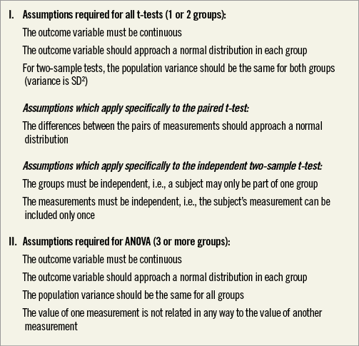
Figure 3. Assumptions for t-test and ANOVA.
Other parametric methods for analysing continuous data, including linear regression, as well as non-parametric methods, will be described in future papers within the current series. Moreover, excellent references on these topics are provided by Bland and Altman5,8.
Conflict of interest statement
The authors have no conflicts of interest to declare.