This article aims to provide an overview of the main concepts of descriptive statistics, which are a fundamental part of data analysis and a prerequisite for the understanding of further statistical evaluations, including inferential statistics. The principal aim of descriptive statistics is to summarise the data, and thus to present the numerical procedures and graphical techniques used to organise and describe the characteristics of a given sample.
The choice of descriptive statistics, and also of statistical analysis, largely depends on the nature of the data being examined. Familiarity with the concepts regarding types of data and data distributions is therefore required for further understanding of statistical concepts.
Types of data
Generally, data can be classified as either numerical or categorical (otherwise known as quantitative and qualitative)1. Numerical data are numerical in nature, while categorical observations are those that are not characterised by a numerical quantity, but whose possible values consist of a number of categories2. Numerical data can be further classified into continuous and discrete variables. Continuous variables can take any value within an upper and lower limit, while discrete numerical data can only take certain numerical values. Examples of continuous numerical variables are weight in kg, systolic blood pressure in mmHg or cholesterol level in mmol/l. An example of a discrete numerical variable is the number of visits to the outpatient clinic in a year. Variables that can be classified into two or more categories are described as categorical variables. If the categorical variable has two categories then it will be called dichotomous or binary. A further classification of a categorical variable is into nominal variables (unordered) and ordinal variables (ordered). Examples of ordinal variables are educational level and NYHA classification. Figure 1 gives a review of types of data, as well as graphs to be used and statistical measures.
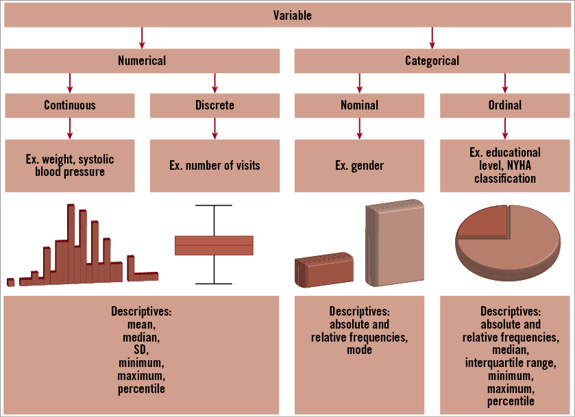
Figure 1. Overview of variable types and suitable statistical measures for descriptive presentation. Adapted from (4).
Descriptive statistics of numerical data
Numerical data can be presented in a graphical way in the form of box plots and histograms. Box plots offer a visual impression of the position of the median (central value), the first and third quartiles (25th and 75th percentile) and minimum and maximum (Figure 2). The box represents the interquartile range (IQR) which includes 50% of the values of distribution. The upper boundary of the box locates the 75th percentile of the data while the lower boundary indicates the 25th percentile. A box with a greater IQR indicates greater scatter of the values. The line in the box indicates the “median” of the data. The “whiskers” of the box plot are the vertical lines of the plot extending from the box, and indicate the minimum and maximum values in the dataset unless outliers are present.
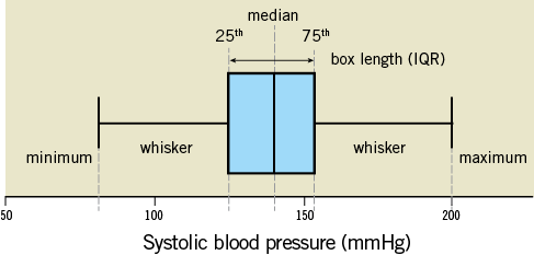
Figure 2. Box plot.
A histogram is a bar chart presenting the number or percentages of observations for each value or group of values (Figure 3). Such graphs give an initial visual impression of the distribution of the collected variables. The smooth curve drawn over the histogram is a mathematical “idealisation” of the distribution. When the smooth curve (or density curve) resembles a symmetrical bell shape, the distribution is called normal. However, when the histogram has a left peak or a right peak, the variable has a skewed distribution. A negative or left skewed distribution has fewer low values and a longer left tail, while a positive of right skewed distribution has fewer high values and a longer right tail (Figure 4).
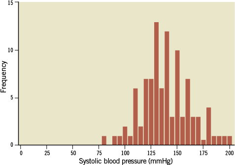
Figure 3. Histogram.
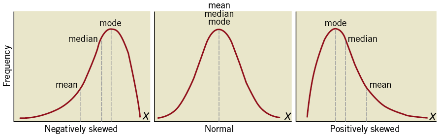
Figure 4. Normal and skewed distributions.
The distribution of continuous variables can be numerically described with measures of central tendency (mean, median and mode) which provide information about the centre of a distribution of values and with measures of dispersion (minimum, maximum, quartiles, and standard deviation) which provide information about the variability of data around the measures of central tendency (Figure 5)3. The arithmetic mean is the average of all values and is calculated by summing all the values and dividing the sum by the number of values. The median is the value that divides the distribution in half, i.e., if the observations are arranged in increasing order, the median is the middle observation. If there is an even number of observations, the average of the two middle ordered values is taken. The mode is defined as the value that appears most often of all observations. Which measures are used to describe a continuous variable depends largely on the distribution of the data. If a variable is symmetrically distributed, e.g., in the case of normal distribution, then the mean, median and mode will be equal (Figure 4). To summarise a variable, it is usually recommended that, when a variable follows a normal distribution, the mean and standard deviation (SD) should be reported (Figure 5). The standard deviation is calculated by taking the square root of the average of the squared differences of the values from their average value. It shows how much variation or dispersion from the average exists. In a normal distribution approximately 95% of cases will have a score within two standard deviations of the mean. If the distribution of values is not symmetrical but skewed, the distribution is characterised by a separation of the mean, median and mode. Using the mean may be unrepresentative of the “mass” of the data in this case. An important feature of the median is that it is not sensitive to outliers and atypical observations. When data are skewed or when their distribution is normal but outliers are present, it is recommended to report the median and interquartile range (e.g., 25th and 75th percentile).
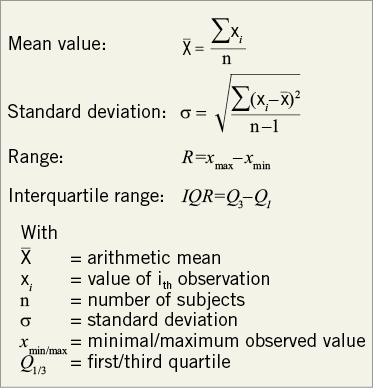
Figure 5. Descriptive statistics.
Descriptive statistics of categorical data
A useful first step in summarising categorical data is to generate frequency statistics2,3. These include absolute frequencies (counts), relative frequencies (proportions and percentages of the total observations) and cumulative frequencies for successive categories of ordinal data. For nominal data the measure of dispersion is based on the frequency of cases in each category. The measure of central tendency for nominal data is the category with the most frequent number of cases, i.e., the mode. The measures of dispersion for ordinal level data are the frequency distribution, percentile and range. As ordinal data are ordered hierarchically, all cases can be sorted from the lowest to the highest score (rank-ordered distribution) and presented with the median.
The bar chart and pie chart are popular graphical presentations for the distribution of categorical variables (Figure 1). The number of segments in one pie diagram corresponds to the number of possible values of the variables, whereas the proportion in the total pie corresponds to their relative percentage. In a bar chart, the frequency values are displayed on the y-axis, which can present absolute or relative frequencies.
Conclusion
Descriptive statistics are an essential part of presenting data. The descriptive presentation includes graphical and tabular presentation of the results. It is important to distinguish between numerical and categorical variables in order to use the appropriate descriptive statistics.
Conflict of interest statement
The authors have no conflicts of interest to declare.