Abstract
Composite endpoints are commonly used in clinical trials, and time-to-first-event analysis has been the usual standard. Time-to-first-event analysis treats all components of the composite endpoint as having equal severity and is heavily influenced by short-term components. Over the last decade, novel statistical approaches have been introduced to overcome these limitations. We reviewed win ratio analysis, competing risk regression, negative binomial regression, Andersen-Gill regression, and weighted composite endpoint (WCE) analysis. Each method has both advantages and limitations. The advantage of win ratio and WCE analyses is that they take event severity into account by assigning weights to each component of the composite endpoint. These weights should be pre-specified because they strongly influence treatment effect estimates. Negative binomial regression and Andersen-Gill analyses consider all events for each patient –rather than only the first event – and tend to have more statistical power than time-to-first-event analysis. Pre-specified novel statistical methods may enhance our understanding of novel therapy when components vary substantially in severity and timing. These methods consider the specific types of patients, drugs, devices, events, and follow-up duration.
Introduction
Composite endpoints are commonly used in clinical trials. Recently, the Academic Research Consortium-2 consensus stated that patient-oriented composite endpoints – the overall cardiovascular outcomes from the patient perspective, including all-cause death, any type of stroke, any myocardial infarction (MI), and any repeat revascularisation – should constitute the foundation of novel coronary device or pharmacotherapeutic agent assessment1.
The time-to-first-event method has been commonly used for the analysis of composite endpoints; however, it has the inherent limitation of treating all contributory endpoints as having equal severity and only gives weight to the first endpoint encountered in time. Thus, non-fatal events that occurred earlier have more impact than more serious events such as stroke or death that occur later. Furthermore, death may preclude or render impossible the observation of non-fatal events.
Over the last decade, several novel statistical methods have been proposed to overcome these limitations. These methods consider all events occurring until follow-up, incorporate the severity of clinical events, and account for the competing risk nature of different events2,3,4,5,6,7,8,9,10,11.
We aimed to review the different statistical methods other than the traditional time-to-first-event analysis, including win ratio analysis, competing risk regression, negative binomial regression, Andersen-Gill regression, and weighted composite endpoint (WCE) analysis (Figure 1).
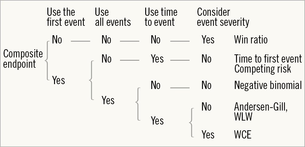
Figure 1. Decision tree for statistical models. WCE: weighted composite endpoint; WLW: Wei-Lin-Weissfel
Statistical approaches
WIN RATIO ANALYSIS
Win ratio analysis was introduced by Pocock et al in 2012 and is a rank-based method, which puts more emphasis on the most clinically important component of the composite endpoints by ranking the constituent components2. This analysis requires four steps: 1) ranking events by their severity, 2) making patient pairs, 3) deciding on a winner in each patient pair, and 4) calculation of the win ratio.
First, the components of the composite endpoint are ranked on the basis of their perceived severity. Second, the concept is to match patients with a different treatment assignment based on their individual risk estimates. Pocock et al proposed estimating a composite risk score for each patient based on pre-selected baseline prognostic factors3. Patients in the experimental treatment arm are matched to patients with a similar risk score in the control arm on the condition that the follow-up durations do not differ greatly (Figure 2A-1). When the number of patients in the two groups differs, some patients are randomly excluded to equalise the number of patients in both groups.
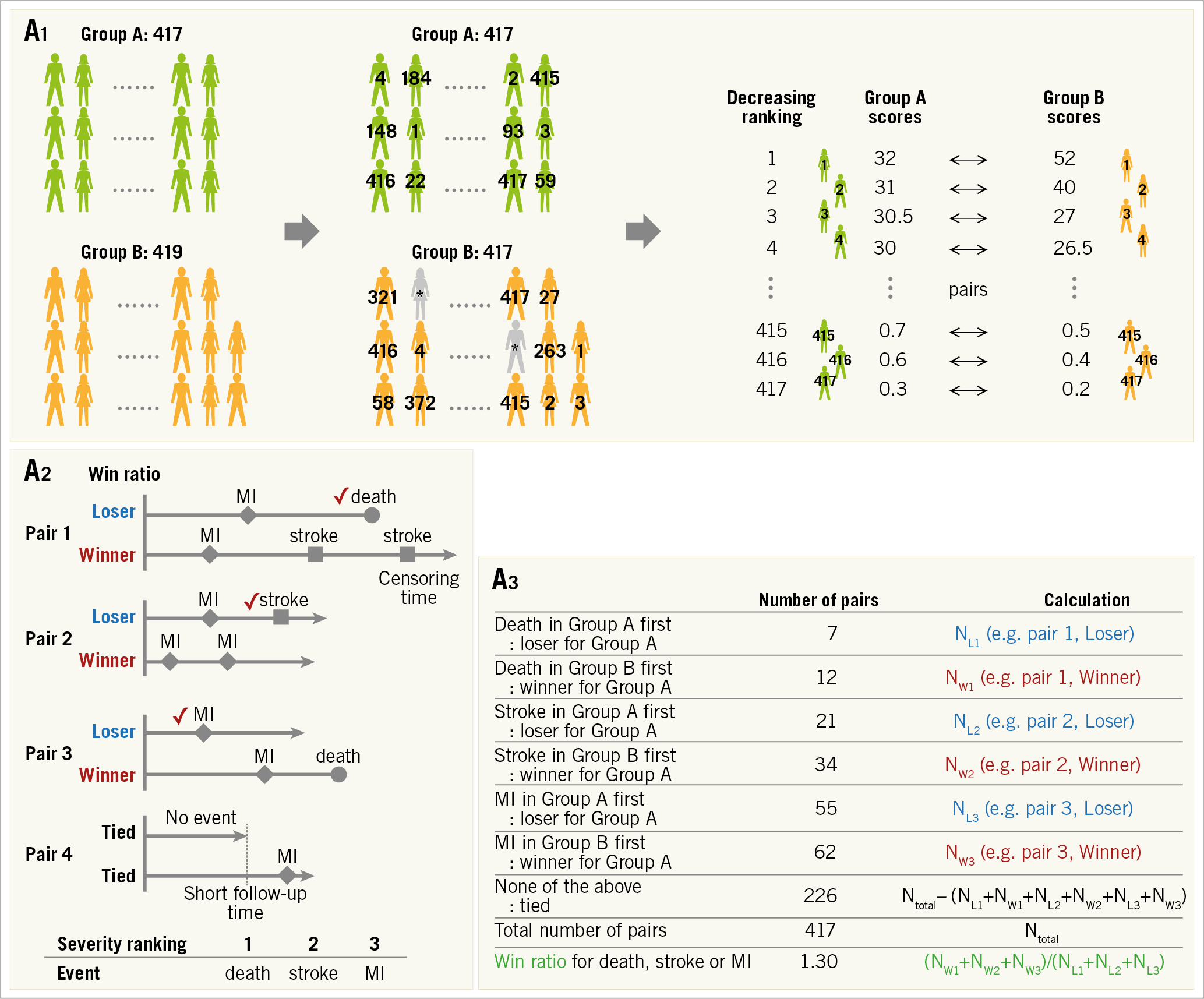
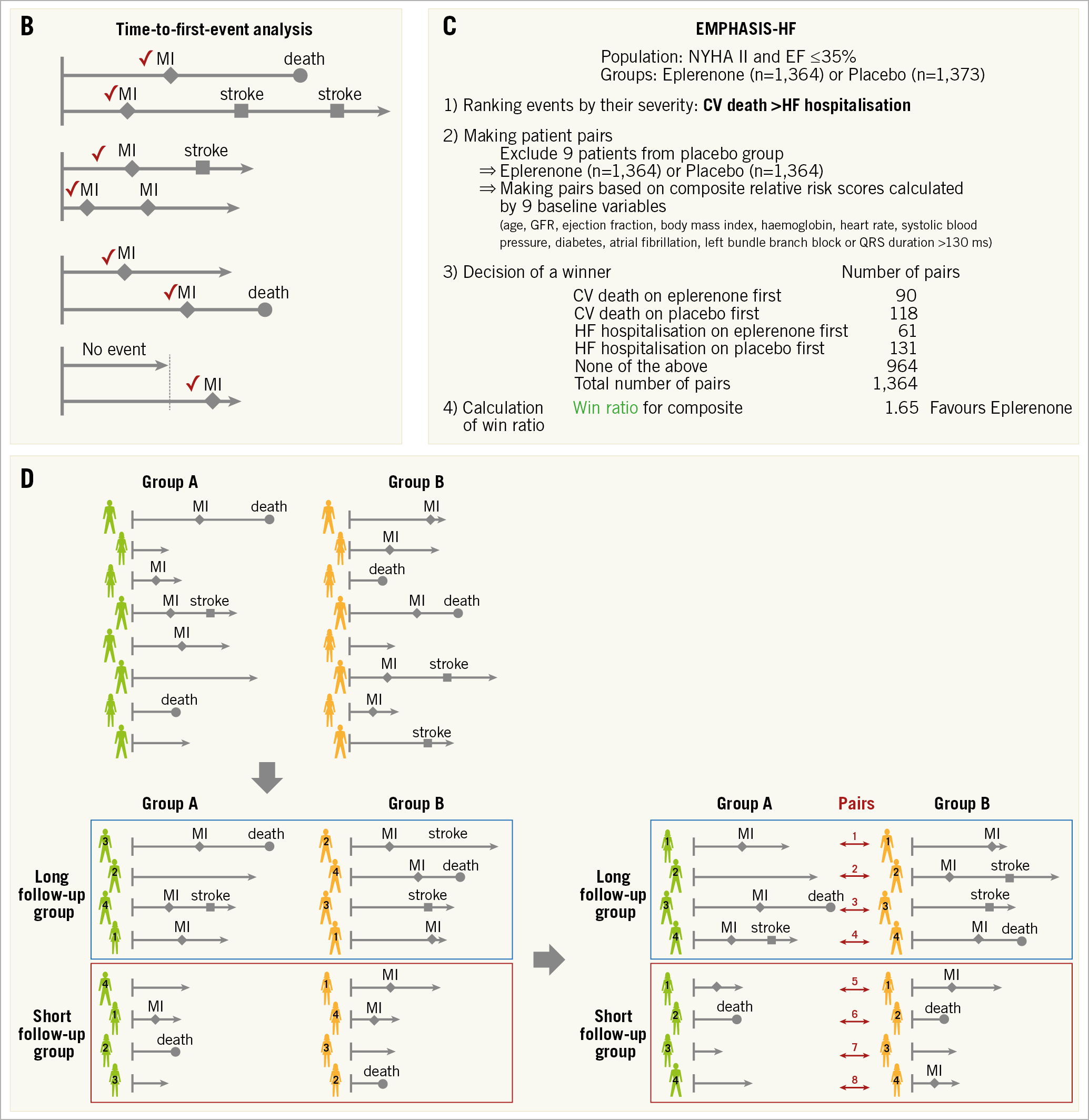
Figure 2. Win ratio. A) Flow chart for analysis. A1. Adjustment of each group. When there are slightly unequal sample sizes in groups A (n=417) and B (n=419), respectively, two patients (*) are randomly excluded from Group B to equalise the number of patients. The patients are arranged and tabulated based on the decreasing ranking of their relative risk scores. A2. Patient level assessment. Winners and losers are decided based on event severity within the censoring period. Provided that the decreasing ranking of event severity is death, stroke and myocardial infarction (MI), decisions in each pair are as follows. (Pair 1) Death is the most severe event, so the patient figuring in the upper line is a loser. (Pair 2) A death does not occur in either patient. The event of stroke should be evaluated because stroke is more severe than MI but less severe than death, and the patient figuring in the upper line is a loser. (Pair 3) A death occurs after the others’ follow-up time, so the times to MI in the absence of death or stroke occurrence should be compared. The upper line patient is a loser. (Pair 4) An MI occurs after the others’ follow-up time, and there are no events until censoring. Therefore, a winner and a loser are not established, and we have a tie. A3. Group assessment. The win ratio is provided by (total number of winners)/(total number of losers). See example: 1.30 (= (12+34+62) / (7+21+55)). Win ratio. B) The events used are different between the win ratio and traditional time-to-first-event analyses. C) The application of win ratio analysis in the EMPHASIS-HF study. D) Time-stratified approach. Whenever patient follow-up durations vary greatly, patients can be stratified into some follow-up duration categories (e.g., long follow-up group and short follow-up group) and pairs are matched in each category based on the decreasing ranking of each patient’s relative risk score. CV: cerebrovascular; EF: ejection fraction; HF: heart failure; NYHA: New York Heart Association
The third step is to decide on a winner in each matched patient pair (Figure 2A-2). The comparison of each pair is performed using every type of categorised event – death, or stroke, or MI, or other event. The events of each patient pair are evaluated to decide whether one had the most severe event (usually death is applied). If this is not the case (both patients were alive at the end of follow-up), the remaining pairs are then evaluated for the occurrence of an event ranked second in severity, and so on for each ranking (third, fourth, or fifth rank). If there were no events until the time of last follow-up, the pair is treated as “tied”2. The win ratio emphasises the more severe components when comparing composite endpoints between two groups of patients (Figure 2A-2 and Figure 2B).
Fourth, the win ratio is calculated as the number of winners divided by the number of losers; a 95% confidence interval for the win ratio is easily obtainable1 (Figure 2A-3). Since matched pairings are influenced by patients who are randomly excluded, it may be necessary to perform analyses repeatedly with different randomly excluded patients. Pocock et al have described the formulas for these calculations2; these calculations do not require special software. In addition, Luo et al presented a code for R software (R Foundation for Statistical Computing, Vienna, Austria) which could be helpful12.
Win ratio analysis is a rank-based method. It could reflect the event severity in the analysis of composite endpoints. Therefore, it is valuable when the components of the composite endpoint vary in their clinical severity and importance (e.g., composite endpoint of death, stroke, MI, and revascularisation in an ischaemic heart disease trial; composite endpoint of cardiovascular death and heart failure hospitalisation in a heart failure trial). On the other hand, there are several limitations. Severity ranking of each adverse event affects the result of the composite endpoint and the ranking in itself is debatable without universal consensus (e.g., severity ranking of MI and major bleeding). In addition, it can only be applied to the comparison between two groups. An example used in the EMPHASIS-HF study, which compared eplerenone (n=1,364) and placebo (n=1,373) in patients with New York Heart Association (NYHA) Class II heart failure and ejection fraction ≤35%, is shown in Figure 2C,2.
Several options for making pairs have been proposed for comparing patients with similar anatomic and physio-pathological backgrounds. For example, prognostic scores, such as the anatomic SYNTAX score and SYNTAX score II, have been applied, instead of composite relative risk scores4,5.
In long-term event-driven trials, patient follow-up durations vary greatly, and many pairs are often categorised as “tied” (Figure 2D). To reduce this problem, patients can be stratified into several follow-up duration categories: patients are matched in strata of similar follow-up duration2.
When baseline risk factors are not well established, it is more difficult to match patients on the basis of risk. In this case, one can compare every patient in one group with every patient in the other group (unmatched pairs approach)2,3.
COMPETING RISK REGRESSION
Events (e.g., non-cardiovascular death) which preclude less severe events or events (e.g., heart transplant) which change the possibility to observe events of interest (e.g., congestive heart failure) are called competing risks (Figure 3A). The competing risk regression method takes these issues into account for composite endpoints and allows disentangling the contribution of an intervention to each type of event. The Fine-Gray model is the most popular model13. In this model, patients experiencing competing risk events remain in the risk set for the event of interest until they experience events of interest or they are censored (Figure 3B, Figure 3C). This analysis can be performed easily using free statistical software (EZR). Kanda has described the method in detail14.
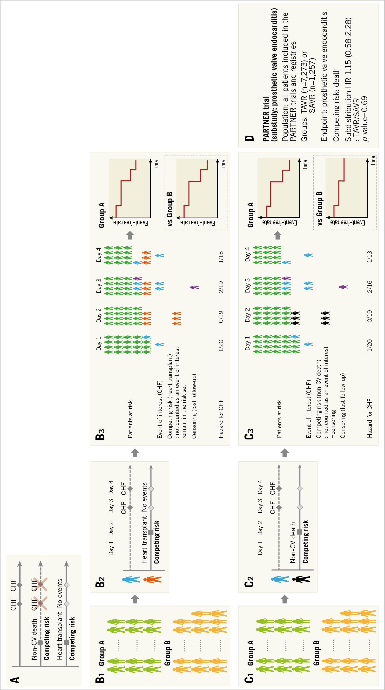
Figure 3. Competing risks. A) Non-cardiovascular (CV) death precludes the possible subsequent events of congestive heart failure (CHF), and heart transplant changes the possibility of CHF occurrence. Therefore, these events are called competing risks. B) Flow chart for analysis. B1. Each group. B2. Patient level assessment. In the Fine-Gray model, patients experiencing competing risk events (e.g., heart transplant) remain in the risk set for the event of interest (e.g., CHF) until either experiencing events of interest or their censoring. B3. Group assessment. From patients at risk and the number of events, the cumulative event rate is calculated. When we compare groups, the result is presented as hazard ratio and p-value. C) Flow chart for analysis. C1. Each group. C2. Patient level assessment. In the case that the competing risk event is a non-CV death, a competing risk event (non-CV death) is treated as a censoring because death is not an event of interest (CHF) and also means the end of follow-up. C3. Group assessment. D) Application of competing risk regression to the sub-analysis of the PARTNER trial. SAVR: surgical aortic valve replacement; TAVR: transcatheter aortic valve replacement
This competing risk within clinical research was first introduced in the field of oncology. In patients who underwent chemotherapy for cancer, failure events commonly studied are relapse of the cancer and treatment-related death. The interest is to estimate the probability of relapse. In this case, treatment-related death is a competing risk event (which would obviously not allow the investigators to observe any relapse of cancer because the patients are dead) and competing risk regression analysis is useful15. When the age of the study population is high, death could be used as a competing risk since the rate of non-treatment-related death is relatively high. In the substudy of prosthetic valve endocarditis from the PARTNER trial16, the age of patients was 83 years and death was used as the competing risk event. The incidence of prosthetic valve endocarditis after transcatheter and surgical aortic valve replacement was assessed using this competing risk regression model (Figure 3D). In the field of cardiology, all-cause death may often be less device- or procedure-specific than deaths adjudicated as cardiovascular death. Non-cardiovascular death could be used as a competing risk, although all-cause death is the most unbiased method to report deaths.
NEGATIVE BINOMIAL REGRESSION
The traditional time-to-first-event analysis only evaluates the first adverse event and does not capture the subsequent events. However, in the field of cardiology, some adverse events, such as revascularisation, bleeding, hospitalisation for heart failure, occur repeatedly. Incorporation of all events is meaningful in terms of the evaluation of patients’ quality of life and medical cost. In addition, an increase in the number of events could yield additional statistical power. A simple method for the assessment of all adverse events between two groups is to compare the number of events.
In a book entitled “The Law of Small Numbers”, Bortkiewicz investigated the annual deaths by horse kicks in the Prussian Army from 1875 to 1894, noting that events with low frequency in a large population follow a Poisson distribution even when the probability varies (Supplementary Figure 1A). The Poisson distribution has commonly been used to model the number of events in an interval of time (Supplementary Figure 1A). The variance of clinical events in a trial is usually greater than the mean (Supplementary Figure 1B). In other words, the distribution of the number of clinical events is better represented by an overdispersed Poisson distribution. The negative binomial distribution is often used for modelling overdispersed Poisson data. Negative binomial regression analysis has been used to estimate treatment effect in terms of the rate ratio of a composite endpoint6,7,8,9 (Figure 4A) and is valuable especially in a high-risk population since patients tend to experience repeated adverse events. For this analysis, the “glm.nb” function from the “MASS” package in R software could be helpful17. In the PARADIGM-HF trial8, the primary endpoint (a composite of cardiovascular death or hospitalisation for congestive heart failure) was analysed by a negative binomial regression analysis (Figure 4B). On the other hand, this analysis considers only the total account of events per patient. Therefore, the same follow-up duration should be applied per patient, which sometimes restricts the application of this method.
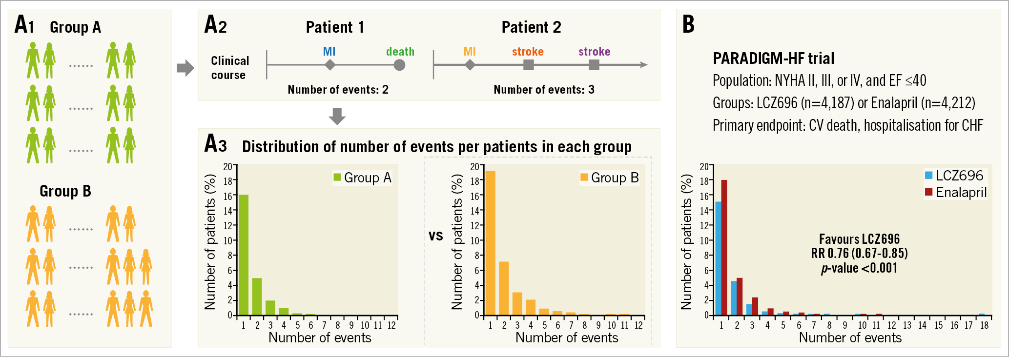
Figure 4. Negative binomial regression analysis. A) Flow chart for analysis. A1. Each group. A2. Patient level assessment. Number of events is counted in each patient. A3. Group assessment. Negative binomial regression is a statistical method for the analysis of overdispersed data. The comparison between groups is shown as rate ratio and p-value. B) Application of negative binomial regression to the PARADIGM-HF trial. CV: cerebrovascular; CHF: congestive heart failure; EF: ejection fraction; NYHA: New York Heart Association; RR: rate ratio
COX-BASED MODELS FOR RECURRENT EVENTS
Negative binomial regression analysis is not applicable if the follow-up duration differs from patient to patient. To overcome this limitation, several time-to-event methods have been proposed for the analysis of repeated events. The Andersen-Gill model is a simple extension of the traditional Cox model and is based on a gap-time approach, in which the clock is reset after an event and the patient is at risk for the next event. This analysis assumes that the risk of an event is not affected by whether another event has already occurred4,5,9. The Wei-Lin-Weissfeld (WLW) model is different from the Andersen-Gill model in that it uses the time from study entry to the first, second and subsequent events (Figure 5A)8,9. In the WLW model, each time-ordered event is analysed on its own time-to-event basis, that is, for the first events in each patient, the second events in each patient, the third events in each patient, and so on. For these analyses, the “coxph” function from the “survival” package in R software could be helpful18. These analyses consider all adverse events and time to events. Therefore, these analyses are valuable in a high-risk population, like the negative binomial regression analysis. In addition, these analyses are applicable regardless of the follow-up duration of each patient. On the other hand, this methodological approach treats all adverse events as having equal severity; severe adverse events, such as death, could be underestimated as well as time-to-first-event analysis. In the REDUCE-IT trial, the primary endpoint (a composite of cardiovascular death, MI, stroke, revascularisation, or hospitalisation for unstable angina) – including recurrent events – was analysed using the Andersen-Gill and the WLW approaches (Figure 5B)9.
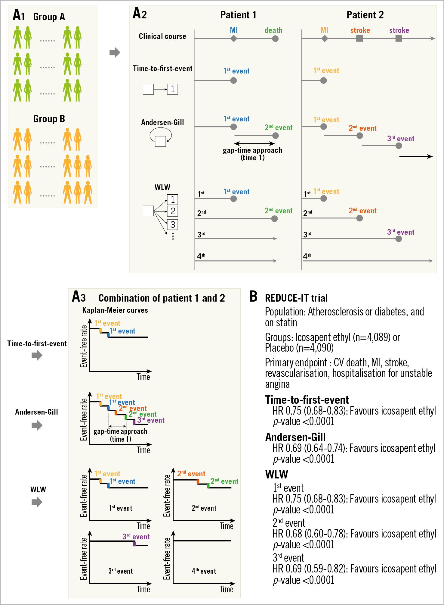
Figure 5. Comparison of time-to-first-event, Andersen-Gill, and Wei-Lin-Weissfeld (WLW) methods. A) Flow chart for analysis. A1. Each group. A2. Patient level assessment. A3. Group assessment. The time-to-first-event analysis uses only the first event and time to the first event. In this example, two step-downs according to the first events in “patient 1” and “patient 2” are shown in the Kaplan-Meier curve. In Andersen-Gill analysis, all events and the times between consecutive events (gap-time approach) are used. Five step-downs according to two events in “patient 1” and three events in “patient 2” are demonstrated in this modified Kaplan-Meier curve. In the WLW method, the analyses for the first events in each patient (e.g., two events in “patient 1 and 2”), the second events in each patient (e.g., two events in “patient 1 and 2”), the third events in each patient (e.g., one event in “patient 2”), and so on (e.g., the fourth event did not occur), are performed. When we compare groups, results are presented as hazard ratios and p-values. B) Application of time-to-first-event, Andersen-Gill, and WLW methods to the REDUCE-IT trial. CV: cerebrovascular; HR: hazard ratio; MI: myocardial infarction
WEIGHTED COMPOSITE ENDPOINT (WCE)
The WCE methodology extends the standard time-to-event methodology by determining a weight for each non-fatal event (event severity) and incorporating all adverse events into the analysis (recurrent events)4,5,10,11. The WCE analysis requires four steps: 1) a decision on event weights, 2) calculation of residual weight at the end of each day in each patient, 3) creation of a modified life table with a weighted number of patients at risk, and 4) comparison of groups (Figure 6A).
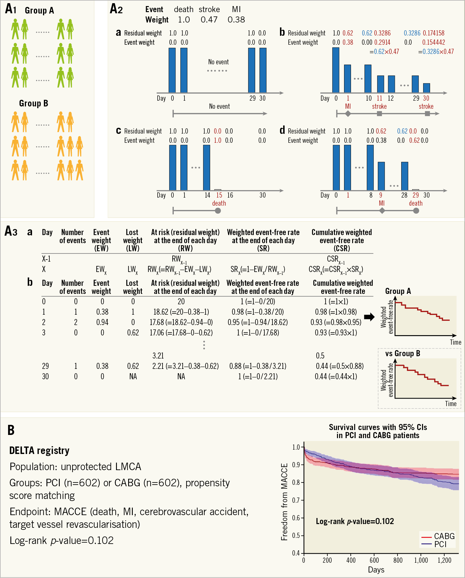
Figure 6. Weighted composite endpoint (WCE). A) Flow chart for analysis. In this explanation, event weights of death, stroke, and myocardial infarction (MI) are assigned as 1.0, 0.47, and 0.38, respectively. A1. Each group. A2. Patient level assessment. The residual weights and event weights in each patient are calculated as follows. (a) No events occur at follow-up, a weight of 1.0 remains unaltered. (b) A patient with a myocardial infarction on day 1 and a non-disabling stroke on day 11 has a cumulative weighting of 0.3286=1–[(1–0.38)×(1–0.47)]. When the patient suffers the second stroke on day 30, the patient has a residual weighting of 0.174158=0.3286×(1–0.47). (c) If a death is the only event, a weight of 1.0 is lost for a death event. (d) If there is an event before a death, the residual weight is lost for a death. A3. Group assessment. (a) Calculation of weighted number of patients at risk (residual weight) and cumulative weighted event-free rate. (b) The table is an example when the number of patients is 20. A modified life table including weighted number of patients at risk and cumulative weighted event-free rate is created from each patient’s data. B) Application of WCE method to the DELTA registry. This figure is reproduced with permission from Capodanno et al3. CABG: coronary artery bypass grafting; CI: confidence interval; LMCA: left main coronary artery disease; MACCE: major adverse cardiac or cerebrovascular events; PCI: percutaneous coronary intervention
In the field of cardiovascular disease, two sets of event weights have been used10,11. The first set gives a weight of 1.0 to death, 0.47 to stroke, 0.38 to MI, and 0.25 to target vessel revascularisation4,5. In the second set, death has a weight of 1.0, shock has a weight of 0.5, congestive heart failure has a weight of 0.3, re-MI has a weight of 0.2, and re-ischaemia has a weight of 0.1. These weights were decided on based on Delphi panels to achieve consensus between clinician-investigators. A Delphi panel is a panel of experts to achieve consensus in solving a problem or deciding on the most appropriate strategy based on the results of multiple rounds of questionnaires.
For calculation of residual weights at each time point, each patient starts with a weight of 1.0, which remains unaltered if no event occurs until the end of follow-up (Figure 6A-2a). Non-fatal events reduce the residual weight of a patient by the weight of the event (Figure 6A-2b, Figure 6A-2c, Figure 6A-2d). From the individual patient data, a modified life table with a weighted number of patients at risk is created, providing estimates of weighted event rates in each group and of a weighted hazard ratio for the reference group (Figure 6A-3). The WCE method allows the incorporation of repeated events in a single patient and distinguishes between the severity of components of the composite endpoint. The indication for this method is the same as that for time-to-first-event analysis. A representative analysis of the WCE in the DELTA registry4 is shown in Figure 6B. This approach may better reflect all event information, but evidently depends on the assigned event weights. Furthermore, weighting events reduces the number of effective events. Therefore, the WCE could limit power and it requires a larger sample size, although statistical power largely depends on severe outcomes, such as death19. To date, commercial statistical software does not support this analysis and there is no R package for this analysis in the Comprehensive R Archive Network or Bioconductor. Therefore, this analysis needs a dedicated program.
Comparison of methods – How do we treat a composite endpoint?
The differences in dealing with composite endpoints are shown in Figure 7. These statistical methods have recently been applied to several clinical trials in the field of cardiology (Figure 8, Figure 9). The estimated treatment effect, using multiple statistical methods, showed similar tendencies but, as expected, the significance of the treatment effect estimates was dependent on the statistical method used in the trials. The negative binomial regression and the Andersen-Gill analyses tended to have more statistical power than time-to-first-event analysis, while the statistical power of the WCE method tended to be low. In particular, the WCE method did not demonstrate a significant difference between treatments (Figure 8), in contrast with time-to-first-event analyses.
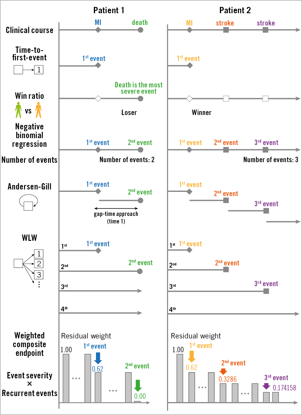
Figure 7. The differences in dealing with composite endpoints. MI: myocardial infarction; WLW: Wei-Lin-Weissfeld
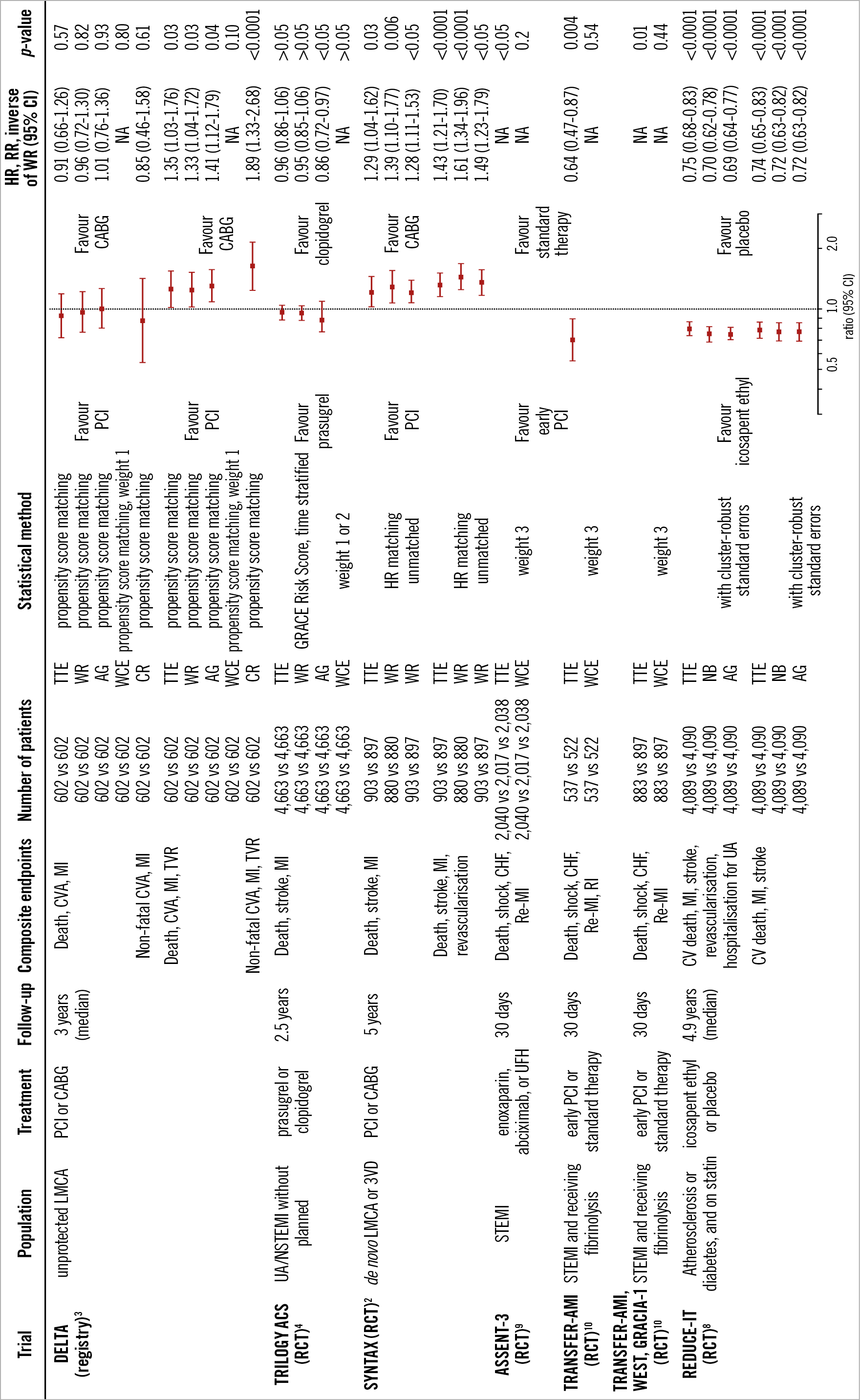
Figure 8. Application of multiple statistical methods to cardiovascular disease trials. Weight 1: death, 1.0; CVA or stroke, 0.47; MI, 0.38; TVR, 0.25. Weight 2: death, 1.0; severe stroke, 0.82; moderate stroke, 0.47; mild stroke, 0.23; severe MI, 0.59; moderate MI, 0.38; mild MI, 0.17. Weight 3: death, 1.0; shock, 0.5; CHF, 0.3; re-MI, 0.2; RI, 0.1. AG: Andersen-Gill; CABG: coronary artery bypass grafting; CI: confidence interval; CR: competing risk; CV: cardiovascular; CVA: cerebrovascular accident; GRACE: Global Registry of Acute Cardiac Events; HR: hazard ratio; LMCA: left main coronary artery disease; MI: myocardial infarction; NA: not available; NB: negative binomial; NSTEMI: non-ST-segment elevation myocardial infarction; PCI: percutaneous coronary intervention; RCT: randomised control trial; re-MI: recurrent myocardial infarction; RI: recurrent ischaemia; RR: rate ratio; STEMI: ST-segment elevation myocardial infarction; 3VD: 3-vessel disease; TTE: time to first event; TVR: target vessel revascularisation; UA: unstable angina; UFH: unfractionated heparin; WCE: weighted composite endpoint; WR: win ratio
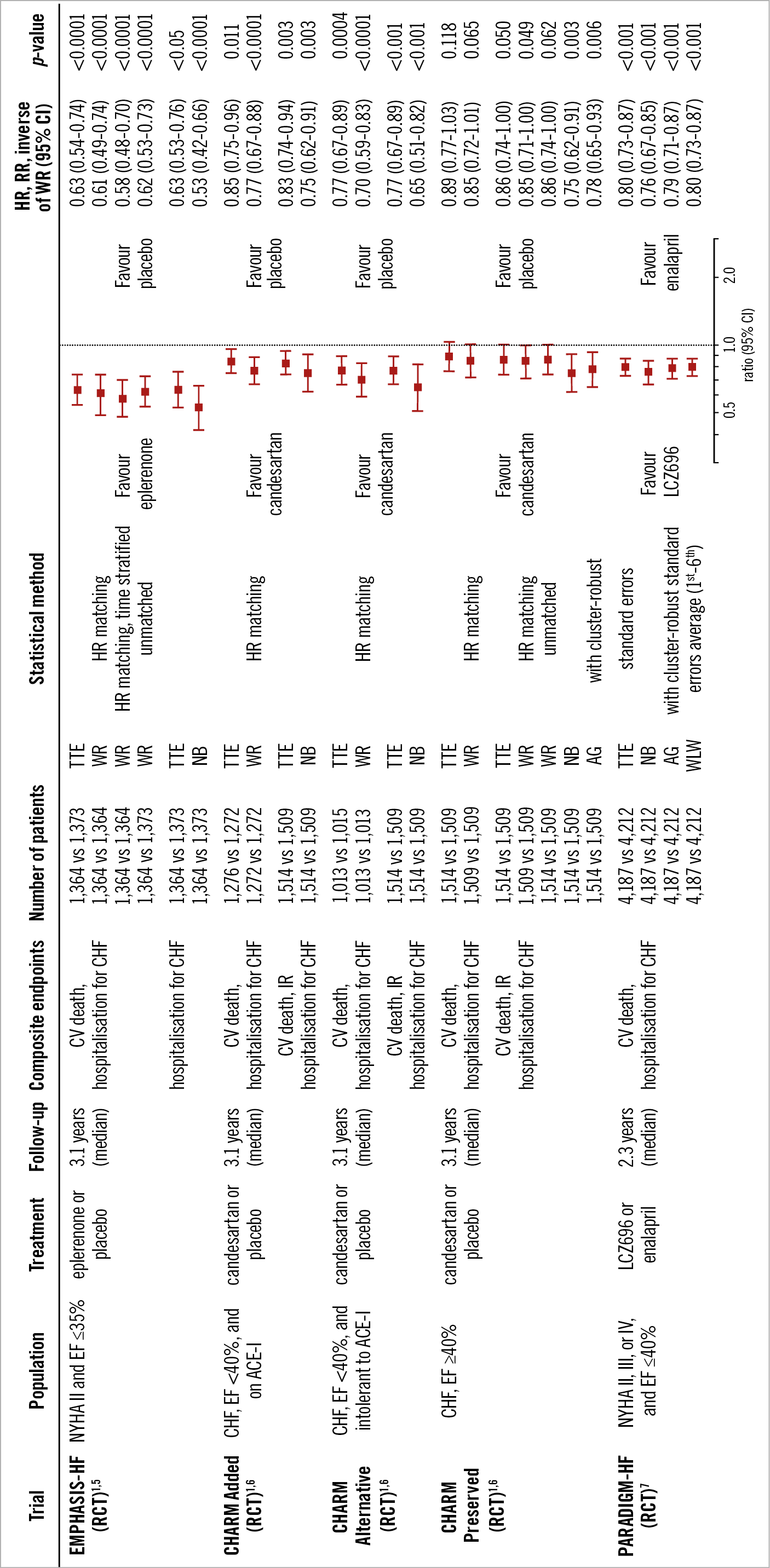
Figure 9. Application of multiple statistical methods to congestive heart failure trials. ACE-I: angiotensin-converting enzyme inhibitor; AG: Andersen-Gill; CHF: congestive heart failure; CI: confidence interval; CVA: cerebrovascular accident; EF: ejection fraction; HR: hazard ratio; IR: investigator reported; NB: negative binomial; NYHA: New York Heart Association; RCT: randomised control trial; RR: rate ratio; TTE: time to first event; WLW: Wei-Lin-Weissfeld; WR: win ratio
The method of counting a “series of events” has to be defined in detail for analyses using all adverse events20. Whenever a revascularisation is performed on the same day as MI, the number of serial events would depend on the methodological definition. Two events (MI and revascularisation) occurring on the same day could even be counted as one event4,9. Therefore, the method of event counting could affect the result.
The win ratio and WCE analyses depend on the severity ranking and weighting of event severity, which may induce arbitrariness of the comparison. On the other hand, a universal ranking is not appropriate because the event severity may depend on patient characteristics. For example, the impact of revascularisation is different in the patients with and without a history of percutaneous coronary intervention. The way to determine event severity should be discussed in future trials. Pre-specification of weights is necessary to avoid any arbitrariness.
Conclusion
All methods for the analysis of composite endpoints have strengths and weaknesses (Figure 10). Pre-specified novel statistical methods may enhance our understanding when components vary substantially in severity and timing. These methods should consider the specific types of patients, drugs, devices, events, and follow-up duration.
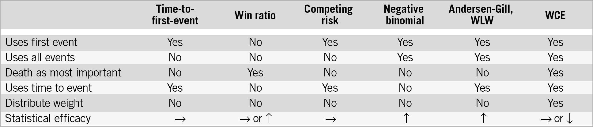
Figure 10. Characteristics of statistical models and statistical power compared to time-to-first-event analysis. WCE: weighted composite endpoint; WLW: Wei-Lin-Weissfeld
Guest Editor
This paper was guest edited by Adnan Kastrati, MD; Deutsches Herzzentrum, Munich, Germany.
Conflict of interest statement
H. Hironori is supported by a grant for studying overseas from the Japanese Circulation Society and a grant from the Fukuda Foundation for Medical Technology. The other authors have no conflicts of interest to declare. The Guest Editor has no conflicts of interest to declare.
Supplementary data
To read the full content of this article, please download the PDF.