Abstract
Propensity score (PS) techniques are useful if the number of potential confounding pretreatment variables is large and the number of analysed outcome events is rather small so that conventional multivariable adjustment is hardly feasible. Only pretreatment characteristics should be chosen to derive PS, and only when they are probably associated with outcome. A careful visual inspection of PS will help to identify areas of no or minimal overlap, which suggests residual confounding, and trimming of the data according to the distribution of PS will help to minimise residual confounding. Standardised differences in pretreatment characteristics provide a useful check of the success of the PS technique employed. As with conventional multivariable adjustment, PS techniques cannot account for confounding variables that are not or are only imperfectly measured, and no PS technique is a substitute for an adequately designed randomised trial.
Introduction
Well-designed large-scale randomised clinical trials (RCTs) are the most reliable approach for investigating the causal effect between an intervention and clinical outcomes. Adequately concealed randomisation1 of several hundred or even several thousand patients ensures that patient groups are almost identical regarding any confounding factors, measured or unmeasured, known or unknown at the time of randomisation. Confounding factors are variables that could distort our interpretation of the presence, direction and magnitude of a true causal effect between interventions and clinical outcomes2. The feasibility of RCTs may be called into question by ethical or economic constraints. The generalisability of results from RCTs may also be limited since the patient population is often highly selected due to restrictive inclusion criteria. In addition, interventions may be more carefully implemented in RCTs, with a high compliance of carers and patients to a standardised protocol, and may not be representative of what is actually implemented in routine clinical settings.
Observational studies are therefore often conducted, either to explore further how results of RCTs translate to routine clinical settings or to obtain information about the effect of an intervention in the absence of RCTs. In these studies, the allocation of patients to treatment groups is based on referral patterns and the clinical reasoning of the therapist. Because the choice of an intervention is probably related to the risk factor of patients, results of observational studies may be confounded. This type of confounding is known as “confounding by indication”3.
Different statistical methods can be used to minimise the influence of confounding by indication. Arguably the most commonly used method, a multivariable regression model, adjusts for patient characteristics (i.e., covariates) that are likely to confound the estimation of the treatment effect. When too many covariates are used for adjustment or the number of outcome events is too small, the validity of multivariable models may be compromised. A rule of thumb suggests that there should be at least 10 outcome events for every covariate included in a multivariable model to prevent overfitting of the model to the data4,5, which results in spurious associations and/or instability of the model.
Propensity score modelling
Propensity score (PS) models may be used to control for confounding by indication even when the number of covariates is large or outcome events are rare. Unlike conventional multivariable adjustments, which model outcomes (i.e., they are based on estimating the association of baseline variables with clinical outcome), PS are based on modelling treatment selection (i.e., they are based on estimating the causal association of pre-treatment variables with interventions). In the typical case there will be considerably more patients who received a given intervention than patients who experienced a given outcome; therefore, the risk of overfitting is smaller for this approach than for conventional multivariable adjustment, which is one of the three major advantages of PS techniques.
A PS quantifies the probability of a patient from zero to one to receive the experimental intervention on which the PS is modelled, given all the pretreatment characteristics included in the model that were used for selecting the treatment a patient received. For instance, in an observational study comparing transcatheter aortic valve implantation (TAVI) with surgical aortic valve replacement (SAVR) in patients with severe aortic stenosis published in 2009 in EuroIntervention, elderly patients and more severely diseased patients were more likely to receive the experimental TAVI than the control SAVR (Table 1)6. The PS model estimates the associations with all relevant variables in a multivariable manner.
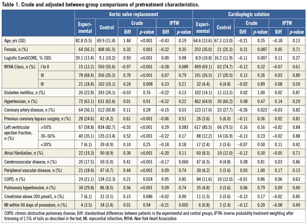
We feel the need to emphasise that the model should include all pretreatment variables that are likely to be associated with the clinical outcome of interest, irrespective of whether they are associated with treatment selection. So, in the example of Table 1, all variables should be used for the PS model, including diabetes mellitus, for example, which does not appear to be associated with the type of intervention (p=0.76), but is certainly associated with the clinical outcome of interest, in this instance overall mortality. Conversely, a variable that is associated with treatment selection, but not with outcome (i.e., an instrumental variable), should not be included in the model7,8. This may seem counterintuitive at first, but makes sense when the aim of PS models is considered: to minimise the effect of confounding on estimating the causal relationship between an intervention and an outcome. If the choice of TAVI, for some esoteric reason, were associated with the signs of the zodiac, this variable should therefore not be included in the model since we do not really have a scientific rationale to suggest that signs of the zodiac are causally related to overall mortality. If it is unclear for a variable that is associated with treatment selection whether it is also associated with outcome or whether it is merely an instrumental variable, we will include it in the PS model7. Technically, a multivariable logistic or probit regression9 with type of treatment as dependent variable and all the pretreatment variables discussed above as independent variables will be used to generate PS. Variables collected at or after treatment initiation absolutely must not be used7,10. These variables need to be considered a result of the treatment decision and can by definition not be causally related to the treatment decision.
Propensity score models eliminate confounding when two conditions are met11. The first condition is that all relevant confounding variables are measured and used to calculate the patients’ PS to receive the experimental treatment. Once all confounding variables are controlled for, the treatment decision itself (before the actual treatment takes place) should no longer predict the outcome. The second condition is that all patients included in the study have a non-null probability to receive either the experimental or control treatment. This means that, at the time of inclusion in the study, all patients had to be potential candidates to receive either of the two compared interventions. This is more or less analogous to patients included in an RCT: only patients who qualify for either of the two compared interventions will be included in the trial, but not those who only qualify for one of the two interventions, but not the other. Only when both conditions are fully met will PS models provide unbiased estimates of the treatment effect.
Visual inspection
Once PS are generated, their distribution can and should be visually inspected. This is the second major advantage of PS techniques. We use smoothed Kernel probability density estimates12,13 of the PS of the two groups to do so, but simple histograms will also do the job. Figure 1A shows the distribution of PS in the above-mentioned comparison of TAVI with SAVR in patients with aortic stenosis6. The distribution of PS in experimental patients receiving TAVI is almost uniformly distributed between zero and one. Conversely, in control patients receiving SAVR, the distribution is completely skewed with a thin long tail towards the right and the Kernel probability density falling to values near null at PS greater than 0.2. So, even if there are few patients with PS between 0.2 and 0.85, which corresponds to probabilities of 20% and 85% of SAVR patients to receive TAVI given their pretreatment characteristics, the thin long tail spread along the null between 0.2 and 0.85 indicates that we cannot be certain that the actual probability of these patients to receive TAVI is anything else but zero.
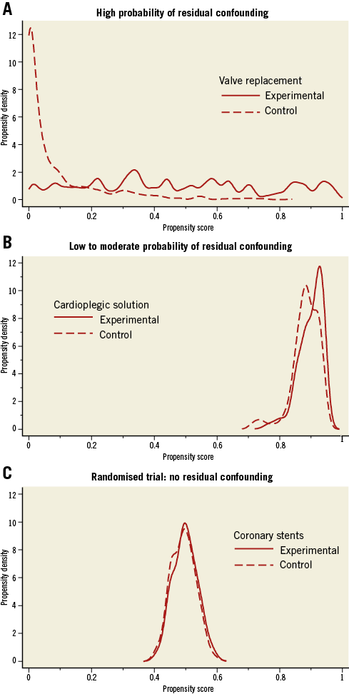
Figure 1. Crude distribution of propensity scores for three clinical examples. A) High probability of residual confounding. B) Low to moderate probability of residual confounding. C) Randomised trial: no residual confounding.
An 81-year-old SAVR patient with a PS of 0.5, for example, may look on paper as if she has had a 50% chance to receive TAVI, but at clinical inspection one would immediately grasp that she appears biologically much younger, has only minor severity of her comorbid conditions, is participating fully in life and shows no signs of frailty, which made her an extremely likely candidate to receive SAVR despite her age and rendered her practically ineligible for receiving TAVI6. In our group, we consider this issue when the Kernel probability density estimate permanently drops below 0.5, but we are not aware of a generally agreed cut-off. In any case, long thin tails of PS that spread near the null point indicate a high probability of residual confounding (here biological rather than chronological age, frailty, severity of comorbid conditions), which may severely distort results, as indeed was the case here6: conventional analyses with multivariable adjustment indicated a threefold increase in the odds of death with TAVI as compared with SAVR (OR 3.05, 95% CI: 1.09 to 8.51) at 30 days6, when the only randomised trial available at the time indicated a trend towards a lower overall mortality at 30 days with TAVI as compared with SAVR (OR 0.53, 95% CI: 0.24 to 1.14)14.
Figure 1B shows the distribution of PS in an observational comparison of two cardioplegic solutions used in patients undergoing SAVR at our centre (unpublished). Compared with Figure 1A, there is a much higher overlap of the distributions of PS between the experimental and control groups, tails are short, Kernel density estimates hardly fall below 0.5, and there is considerably less asymmetry of the two distributions than observed in Figure 1A for SAVR patients. While we acknowledge that the data are observational in nature and therefore distortion of results through residual confounding is always possible, we deem residual confounding considerably less likely here than in the first example. For further comparison, we show the optimal distribution of PS, as derived from a randomised trial (Figure 1C). Here, we calculated PS for being treated with an experimental coronary stent as compared to a control stent in patients with acute myocardial infarction in a trial with a 1:1 randomisation15. PS of both groups scatter around 0.5, corresponding to a 50% chance to receive an experimental stent, with a narrow, symmetrical distribution and near superimposition of scores of the two groups.
Propensity score trimming
A logical consequence from the reasoning above is to drop patients with PS in areas suspected of residual confounding by trimming the tails at both ends of the distribution, which is the third major advantage of PS models. Figure 2 shows this for the observational comparison of cardioplegic solutions. Here, the larger value of the 2.5th percentile of the PS was found at 0.797 in the experimental group, while the smaller value of the 97.5th percentile was found at 0.937 in the control group. Observations in both groups that have PS beyond these two cut-offs are dropped16. We do not advocate trimming based on the common support assumption, even though we previously used it6, since the cut-off will depend heavily on the parameters used for the Kernel probability density function12,13. After trimming, the study population becomes more selected and, again analogous to an RCT, results after trimming may not be generalisable to all patients seen in routine clinical practice.
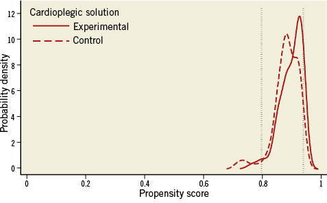
Figure 2. Trimming of propensity score distributions in both groups with cut-offs below the 2.5 percentile in the experimental group and above 97.5 percentile in the control group for the comparison of cardioplegic solutions.
Use of propensity scores for adjustment
After PS are estimated, they can be incorporated in regression models used to estimate the treatment effect as specified in Table 2. We mostly use matching on PS or inverse probability of treatment weighting (IPTW). For matching, we advocate 1:1 or 1:n nearest neighbour matching within a calliper of a fifth of the pooled standard deviation of the PS observed in the two groups after trimming. If the pooled standard deviation of the PS is 0.15, for example, we use a calliper width for matching of 0.03 on the PS scale, which ranges from zero to one. Using this approach for the logit of the PS rather than the PS may even be preferable17. Callipers should not be chosen too narrow, since this will lead to an unnecessary loss of observations. Matching should be accounted for in the analysis, such as the use of a Cox proportional hazards model for time to event data stratified by matched pairs18, or conditional logistic regression for binary data.
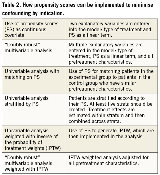
Figure 3 presents the distribution of PS after 1:1 matching. Figure 3A shows a multimodal distribution for the TAVI versus SAVR comparison, which suggests instability of the approach even though matching worked perfectly and the distribution of PS scores from experimental and control groups are nearly superimposed. This suspicion is confirmed when using 1:1 matching for the analysis of 30-day mortality, since we still find completely biased results: an OR of 5.00 (95% CI: 0.58 to 42.8) when the best estimate from an RCT is 0.5314. Conversely, the distribution of the PS of the comparison of cardioplegic solutions after 1:1 PS matching (Figure 3B) looks much like the distribution found in the randomised trial (Figure 3C), which suggests that we can be rather confident when interpreting results of the 1:1 matched comparison of cardioplegic solutions.
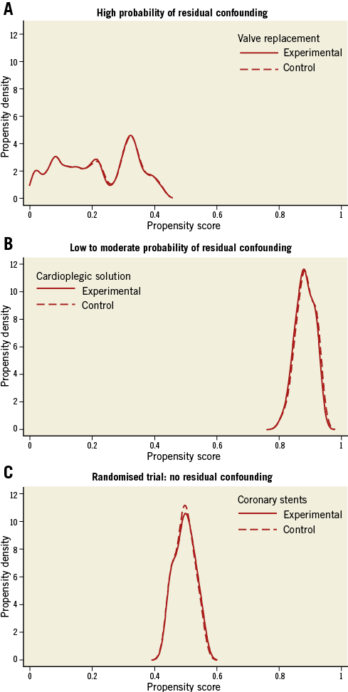
Figure 3. Distribution of propensity scores after trimming and 1:1 matching. A) High probability of residual confounding. B) Low to moderate probability of residual confounding. C) Randomised trial: no residual confounding.
A disadvantage of PS matching, particularly when using a ratio of 1:1, is the loss of observations. Therefore, we perform weighted univariable analyses using inverse probability of treatment weights (IPTW) more and more often19. IPTW analyses use the inverse of the propensity score as weights in patients who received the experimental intervention and the inverse of one minus the propensity score in patients who received the control intervention (assuming that PS is modelled on the experimental intervention). Patients who had a low probability of receiving the experimental intervention but received it anyway will be upweighted in the analysis, whereas patients with a high probability of receiving the experimental intervention who actually received it will be downweighted in the analysis. An alternative to IPTW, which also avoids the loss of observations, is stratification of the analysis by PS. For this purpose, PS should be stratified at least in quintiles20. If the number of observations is large, even smaller strata can be used. For an extended description of the different methods, see Heinze and Jüni21. Doubly robust methods essentially combine multivariable adjustment with PS methods. Two simple approaches are also specified in Table 2. Our group has only little experience with these approaches6, and we are unaware of clear evidence to suggest that these methods are superior to PS matching and IPTW.
Comparison of pretreatment characteristics
Once the PS model is implemented, its success in minimising imbalances in pretreatment characteristics needs to be checked. For this purpose, standardised differences will be calculated, dividing the difference in arithmetic means or the difference in proportions by the respective pooled standard deviation. Differences are expressed as standard deviation units and interpreted as effect sizes, as classically described by Cohen22: ±0.20 standard deviations difference represent a small biological difference, ±0.50 a moderate and ±0.80 a large difference. If a PS technique is successful, one would expect standardised differences of ±0.10 standard deviation units or less, which is considered an irrelevant difference.
Table 1 presents a comparison of pretreatment characteristics of patients included in the comparison of TAVI versus SAVR6, which was characterised by the grotesquely skewed distribution of PS in SAVR patients and minimal or no overlap of PS with the majority of TAVI patients (Figure 1). The crude analysis of pretreatment characteristics of all patients shows dramatic differences, with four standardised differences beyond ±0.80, five beyond ±0.50, and another five beyond ±0.20. Unsurprisingly, 14 differences are statistically significant at p<0.05. The IPTW model used after trimming for calculating adjusted standardised differences improves the situation somewhat, but nine standardised differences are still beyond ±0.20, even though only one is statistically significant, which suggests residual baseline imbalances. Of these, six change sign, which additionally suggests instability of the approach and untrustworthy results. This time, the OR of 30-day mortality is 1.87 (95% CI: 0.50 to 6.99), which appears less biased than results from the PS matched analysis above, but still at odds with the randomised trial14. Even though the previously used approach towards trimming did not differ much from the approach discussed here, results of the corresponding IPTW analysis were completely different (OR 0.35, 95% CI: 0.04 to 2.72)6.
Table 1 presents a comparison of pretreatment characteristics of patients included in the comparison of cardioplegic solution. Here, crude standardised differences are considerably less pronounced than in the previous example, and IPTW analysis after trimming yields minimal standardised differences, with none beyond ±0.20 and only one beyond ±0.10. Together with Figure 3B, which shows a distribution of PS much like that from an RCT, this suggests that we can be reasonably confident of the results yielded by PS techniques in this example.
Conclusion
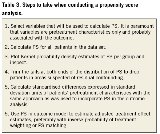
In conclusion, PS techniques are useful if the number of potential confounding pretreatment variables is large and the number of analysed outcome events is rather small so that conventional multivariable adjustment is hardly feasible. The steps to take when performing a PS analysis are specified in Table 3. Only pretreatment characteristics should be chosen for the PS model, and only when they are probably associated with outcome. A careful visual inspection of PS will help to identify areas of no or minimal overlap, which suggests residual confounding, and trimming of the data according to the distribution of PS will help to minimise residual confounding. Standardised differences in pretreatment characteristics provide a useful check of the success of the PS technique. As with conventional multivariable adjustment, PS techniques cannot account for confounding variables that are not or are only imperfectly measured, and no PS technique is a substitute for an adequately designed randomised trial.
Conflict of interest statement
CTU Bern, which is part of the University of Bern, has a staff policy of not accepting honoraria or consultancy fees. However, CTU Bern is involved in design, conduct, or analysis of clinical studies funded by Abbott Vascular, Ablynx, Amgen, AstraZeneca, Biosensors, Biotronik, Boehringer Ingelheim, Eisai, Eli Lilly, Exelixis, Geron, Gilead Sciences, Nestlé, Novartis, Novo Nordisc, Padma, Roche, Schering-Plough, St. Jude Medical, and Swiss Cardio Technologies. P. Jüni is an unpaid steering committee or statistical executive committee member of trials funded by Abbott Vascular, Biosensors, Medtronic and Johnson & Johnson. The other authors have no conflicts of interest to declare.
