Abstract
Aims: Optical coherence tomography (OCT) of a bioresorbable vascular scaffold (BVS) produces a highly reflective signal outlining struts. This signal interferes with the measurement of strut thickness, as the boundaries cannot be accurately identified, and with the assessment of coverage, because the neointimal backscattering convolutes that of the polymer, frequently making them indistinguishable from one another. We hypothesise that Gaussian line spread functions (LSFs) can facilitate identification of strut boundaries, improving the accuracy of strut thickness measurements and coverage assessment.
Methods and results: Forty-eight randomly selected BVS struts from 12 patients in the ABSORB Cohort B clinical study and four Yucatan minipigs were analysed at baseline and follow-up (six months in humans, 28 days in pigs). Signal intensities from the raw OCT backscattering were fit to Gaussian LSFs for each interface, from which peak intensity and full-width-at-half-maximum (FWHM) were calculated. Neointimal coverage resulted in significantly different LSFs and higher FWHM values relative to uncovered struts at baseline (p<0.0001). Abluminal polymer-tissue interfaces were also significantly different between baseline and follow-up (p =0.0004 in humans, p <0.0001 in pigs). Using the location of the half-max of the LSF as the polymer-tissue boundary, the average strut thickness was 158±11 µm at baseline and 152±20 µm at six months (p=0.886), not significantly different from nominal strut thickness.
Conclusions: Fitting the raw OCT backscattering signal to a Gaussian LSF facilitates identification of the interfaces between BVS polymer and lumen or tissue. Such analysis enables more precise measurement of the strut thickness and an objective assessment of coverage.
Introduction
The ABSORB™ bioresorbable vascular scaffold (BVS) (Abbott Vascular, Santa Clara, CA, USA) consists of a semi-crystalline poly(L-lactide) (PLLA) backbone and conformal coating of amorphous poly(D,L-lactide) (PDLLA) and the antiproliferative agent everolimus. The ABSORB BVS struts are fully resorbed approximately two years after implantation,1,2 following a process in which the long chains of PLLA and PDLLA are progressively shortened as the ester bonds present in each lactic acid repeat unit are hydrolysed. Ultimately, PLLA and PDLLA degrade to lactic acid, which is metabolised via the Krebs’ cycle.3 ABSORB has exhibited excellent clinical and angiographic results up to two years follow-up.1,4
A BVS is particularly suitable for optical coherence tomography (OCT) imaging, given the translucency of the polymers from which it is manufactured. The transmitted light can readily penetrate the material and any backscattering stems from changes in refractive index on a length scale greater than or equal to the wavelength of the light. Immediately post-implantation, backscattering associated with the BVS is only significant at the borders of the strut, and changes in backscattering at later time points suggest an evolution in polymer microstructure on the length scale described above. Struts imaged with OCT post-implantation typically appear as a box-shaped highly reflective frame that marks the refractive index change at the lumen-polymer and polymer-tissue interfaces.1,4 However, measuring the strut thickness from leading-edge to leading-edge of the adluminal and abluminal boundaries of this frame results in values greater than the nominal 158 μm value characteristic of the backbone and coating of the ABSORB BVS strut. This discrepancy highlights a lack of precision in the measurement and the need to develop a methodology by which OCT signals may be used to accurately discern the true edges of BVS struts. Even histological assessment may not provide accurate strut measurements at all-time points due to processing artifacts,2 reinforcing the importance of improving the accuracy of OCT measurements.
OCT is an experimental tool for the evaluation of neointimal coverage after implantation of metallic stents5-10 and translucent polymeric scaffolds.2 Coverage assessed by OCT in vivo correlates well with neointimal coverage assessed by histology in experimental animal models.2,5-10 Unlike metallic stents, the assessment of coverage in the ABSORB BVS is more challenging, because the backscattering from thin neointimal layers mixes with that from the polymer interface and can be difficult to discern in a conventional analysis of the log-transformed OCT signal.
The basic principles of light and its interaction with matter provide the means by which these challenges may be addressed. A point spread function (PSF) describes the response of an imaging system to a point source or point object. Similarly, the spreading of light along a perfect line or slit has been called the line spread function (LSF).11 Because OCT is a measurement of backscattering intensity, the edge of a BVS strut forms a relatively uniform line from which a LSF can be measured. However, when tissue or other backscattering media are present, the uniformity of the optical response at the edge may vary. By smoothing the edge response variance due to backscattering tissue, the LSF may facilitate the definition of BVS strut edges and provide an objective criterion for the measurement of strut thickness and tissue coverage.
Methods
Clinical study
The ABSORB Cohort B study (NCT00856856) design has been published elsewhere.12 It enrolled patients older than 18 years with diagnosis of stable or unstable angina pectoris or silent ischaemia and de novo lesions in native coronary arteries amenable to percutaneous treatment with the ABSORB BVS. Target lesions were required to be characterised by percent diameter stenosis greater than or equal to 50% by visual estimation and reference vessel diameter of 2.5-3.5 mm. Major exclusion criteria were: acute myocardial infarction, unstable arrhythmias, left ventricular ejection fraction less than or equal to 30%, restenotic lesions, lesions located in the left main coronary artery or in bifurcations involving a side branch greater than 2 mm, a second clinically or haemodynamically significant lesion in the target vessel, documentation of intracoronary thrombus, or initial TIMI 0 flow. All the study lesions were treated with the ABSORB BVS revision 1.1 (3.0×18 mm). Fifty percent of the cohort underwent scheduled invasive follow-up six months after the implantation, including OCT study whenever available at the participating site. The registry was approved by the ethics committee at each participating site, and each patient gave written informed consent before inclusion in the study.
Preclinical (porcine) study
All experimentation conformed with the Animal Welfare Act, the Guide for Care and Use of Laboratory Animals (NIH Publication 85-23, 1996), and the Canadian Council on Animal Care regulations. All procedures were performed at AccelLab, Inc. (Montreal, Quebec, Canada), accredited by the Association for Assessment and Accreditation of Laboratory Animal Care (AAALAC) and in accordance with the protocol approved by the institutions animal care and use committee (IACUC).
Four Yucatan mini-swine implanted with BVS were used in this analysis. Animals were administered oral acetylsalicylic acid (325 mg initial dose, 81 mg daily subsequently) and clopidogrel (300 mg initial dose and 75 mg daily subsequently) beginning three days prior to BVS implantation. Animals were tranquilised with ketamine (0.04 mg/kg), azaperone (4.0 mg/kg), and atropine (25 mg/kg) intramuscularly. Anaesthesia was achieved with propofol, (1.66 mg/kg IV), and maintained with inhaled isofluorane (1-3%) throughout the procedure. A vascular access sheath was placed in the femoral artery percutaneously. Before catheterisation, heparin (5,000 to 10,000 U) was injected to maintain an activated clotting time greater than 250 s. For each BVS deployment, an arterial segment was chosen so as to achieve a balloon-to-artery ratio of 1.1:1, ensuring full apposition based on angiographic assessment. Each animal received a single BVS revision 1.1 in one of the three main coronary arteries. Although a 3.0×12 mm BVS was used in the animal studies, the design was the same as that used in the clinical study. Animals recovered from anaesthesia under veterinary care for future time point analysis following the procedure. All the devices were imaged by OCT immediately after implantation and at 28-day follow-up.
OCT image acquisition and analysis
In both animal and human procedures, OCT pullbacks were obtained at baseline and follow-up with a Fourier-domain C7 system using a Dragonfly™ catheter (St. Jude Medical Inc., Saint Paul, MN, USA) 10-15 μm axial and 20-40 μm lateral resolution13 at a rotation speed of 100 frames/s with non-occlusive technique.14 After infusion of intracoronary nitroglycerine, the imaging wire was withdrawn by a motorised pullback at a constant speed of 20 mm/s, while Iodixanol 320 contrast (Visipaque™, GE Health Care, Cork, Ireland) was infused through the guiding catheter at a continuous rate of 2-4 mL/min.
A random sampling of 12 struts at each time point from both the animal and the human studies was selected using the following criteria: (1) OCT images were obtained with a Fourier-domain C7 system at both baseline and follow-up; (2) the luminal edge of the strut was perpendicular to the light source in order to minimise the effect of wire eccentricity and vessel-catheter misalignment; and (3) the strut was well-apposed.
Light intensity analysis was performed in the region surrounding the selected struts using ImageJ 1.43 u software (Wayne Rasband, National Institutes of Health, USA). The raw polar image was used to ensure that interpolation, dynamic range compression, or other image processing did not alter the signal and bias the analysis. Because the strut boundaries are expected to be found within the reflective frame, an intensity profile was created by averaging consecutive pixels aligned parallel to the frame boundary and spanning the whole reflective frame orthogonally through the frame boundaries beginning on the adluminal side. Since the C7 system displays 500 A-lines per frame, 976 pixels per line, and a depth of field 5 mm, the axial dimension of a single pixel in raw polar coordinates is ca. 5.12 µm for in vivo coronary imaging with this OCT catheter. Using the catheter dimensions as a standard (0.89 mm), we measured the pixel/µm conversion factor at 5.05 µm and used this for the measurements herein. The result is a two-dimensional profile plot of intensity versus distance through the centre of the strut. The following interfaces were analysed (Figure 1): lumen-polymer, defined as the optical signal generated by the adluminal border of the strut at baseline (LP-bl); lumen-neointima-polymer, defined as the optical signal generated by the adluminal border of the strut at follow-up (LNP-fu); polymer-vessel wall, defined as the optical signal generated by the abluminal border of the well-apposed strut at baseline or follow-up (PV-bl; PV-fu); lumen-vessel wall, defined as the optical signal generated by the vessel wall of a strut-free sector at baseline or follow-up (LV-bl; LV-fu).
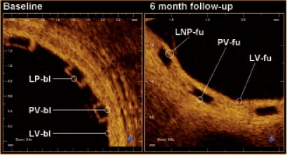
Figure 1. Denomination of the different optical interfaces analysed. LNP-fu: lumen-neointima-polymer at follow-up; LP-bl: lumen-polymer at baseline; LV-bl: lumen-vessel at baseline; LV-fu: lumen-vessel at follow-up; PV-bl: polymer-vessel at baseline; PV-fu: polymer-vessel at follow-up
The data corresponding to each interface were individually summarised in plots of optical intensity versus distance, where the origin of the plot was located at the point corresponding to the strut centre and zero optical intensity (Figure 2). The centre of the strut was determined as the point equidistant from the points at which the intensity signal exceeded a consistent threshold value at the strut interior side of the adluminal and abluminal interfaces.
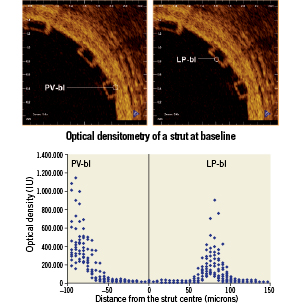
Figure 2. Graphic representation of the 12 struts analysed at baseline. The coordinate system origin is located at the calculated centre of the strut (x-axis) and zero optical intensity (y-axis). The strut centre is defined as the point equidistant to the rises of the adluminal (LP-bl interface) and abluminal (PV-bl interface) strut borders. LP-bl: lumen-polymer interface at baseline; PV-bl: polymer-vessel interface at baseline
The curves for each type of interface were fit to a Gaussian form given by:
 ,
,
where a is the maximum intensity of the curve, b is the midpoint of the Gaussian curve, and c is a function of the full-width-at-half-maximum (FWHM), namely  . Coefficients for the Gaussian curve fits were determined using an iterative least squares minimisation process (Figure 3). Gaussian curves were chosen to remain consistent with the practice commonly used for PSFs. Because the LSF differs from the PSF and includes scattering components, other functions commonly used to describe optical profiles, Lorentzian and exponential functions15-17, were also evaluated and found inferior to the Gaussian fits (data not shown). Where tissue was present, the LSF was derived through symmetry of a one-tailed Gaussian fit with the first peak defining the peak of the Gaussian function. Though the transition between polymer and tissue appears to be sigmoidal or step-like, mirroring a one-sided Gaussian function enabled comparison with the Gaussian fit of the uncovered strut. Additionally, the convolution of two Gaussian functions is a Gaussian function, and thus this best represented the optics of the system.
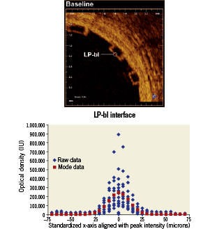
Figure 3. Lumen-polymer interface curve fit. LP-bl: lumen-polymer interface at baseline
Two approaches were used to determine the location of strut interfaces. For struts without tissue coverage (e.g., LP-bl), the strut interface was assigned to the location of the peak of the signal intensity. The justification is that the high signal contrast of the LP interface represents an ideal LSF example, and the peak of the LSF defines the line. Alternatively, for interfaces adjacent to tissue (e.g., LNP-fu, PV-bl, PV-fu, LV-bl, LV-fu), the location of the half-max was assigned to the interface to represent the spatial location of intensity halfway between the low polymer intensity and high tissue intensity18. Because there was no normalisation of the intensity signal, the half-max was chosen to enable objective threshold based filtering. All strut width measurements were performed according to these definitions.
Statistical analysis
Non-linear least squares curve fits were compared with a Snedecor F-test using sum of squares for two separate curves and sum of squares of a single curve generated from combined data. Strut width measurements were compared using a two tailed Fisher’s student t-test. All the analysis was performed with Microsoft Excel 2003, SP3 with solver toolkit.
Results
Results in human
Twenty-four patients in the ABSORB Cohort B study received OCT at baseline and 6-month follow-up. In only 12 of these cases were the images acquired with a Fourier-domain C7 system. One strut meeting the selection criteria of the study was randomly selected for each OCT pullback (12 at baseline, 12 at follow-up).
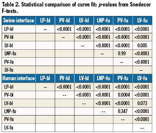
Across all types of interface, the FWHM of the signal was greatest for LV-fu (56.91 µm) and least for LP-bl at baseline (25.86 µm). Table 1 summarises the curve fit parameters for each interface type (Figures 4 and 5). Neointimal coverage of struts resulted in an increase of the FWHM, and the curves corresponding to LP-bl and LNP-fu interfaces differed significantly (p<0.0001, Table 2). There was no significant difference between LNP-fu and PV-fu interfaces (LNP-fu vs. PV-fu, p=0.347). However, the PV-bl interface differed significantly from the PV-fu interface (PV-bl vs. PV-fu, p=0.0004) as well as the LV-bl, LV-fu, and LPN-fu interfaces (PV-bl vs. LV-bl, p<0.0001; PV-bl vs. LV-fu, p<0.0001; PV-bl vs. LPN-fu, p<0.0001).
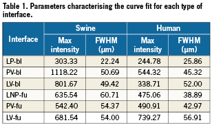
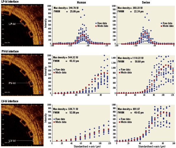
Figure 4. Fitting curves characterising the different interfaces at baseline in human and swine studies. FWHM: full width at half max; LP-bl: lumen-polymer at baseline; LV-bl: lumen-vessel at baseline; PV-bl: polymer-vessel at baseline
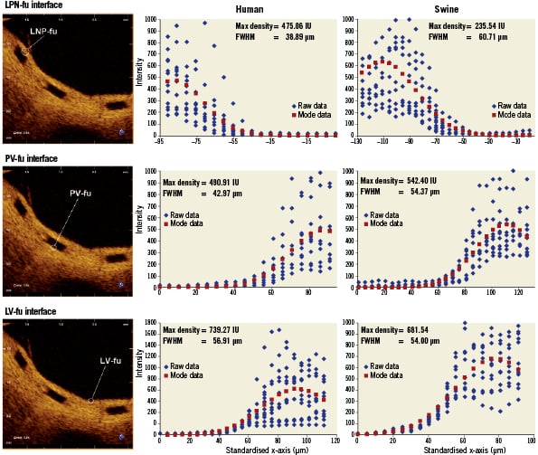
Figure 5. Fitting curves characterising the different interfaces at follow-up in human (6 months) and swine (28 days) studies. FWHM: full width at half max; LNP-fu: lumen-neointima-polymer at follow-up; LV-fu: lumen-vessel at follow-up; PV-fu: polymer-vessel at follow-up
Measuring from peak to half-max (PV-bl to PV-bl) and half-max to half-max (LNP-fu to PV-fu) for baseline and follow-up, respectively (Figure 6), the average strut thickness was 158±11 µm at baseline and 152±20 µm at the 6-month follow-up (p=0.41), both of which are similar to the nominal BVS strut thickness (ca. 152 µm for the backbone only and ca. 158 µm for the backbone and coating).
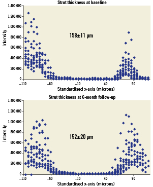
Figure 6. (A) Strut thickness measured from the peak intensity of the fitting curve for the adluminal interface to the half-max of the fitting curve for the abluminal interface at baseline, and (B) strut thickness measured from the half-max of the fitting curve for the adluminal interface to the half-max of the fitting curve for the abluminal interface at follow-up (human data).
Results in the swine model
Three struts meeting the same selection criteria defined for the clinical sample were randomly selected in each of the four animals (12 at baseline, 12 at follow-up). The curve fit parameters for each interface had absolute values different than the ones reported in humans, but the same trends were observed.
Similar to the clinical samples, the FWHM increased when tissue was present. In swine samples, LNP-fu had the greatest FWHM at 60.71 µm, while LP-bl had the smallest FWHM at 22.24. Table 1 summarises the curve fit parameters for each interface (Figures 4 and 5). Neointimal coverage of struts resulted in an increase of the FWHM when going from LP-bl to LNP-fu (p<0.0001, Table 2). Paralleling the human results, the LNP and PV interfaces had similar FHWM at the 28-day follow-up. All other curves were significantly different from each other with p values less than 0.01.
Based upon the previously defined edge detection algorithm, the average strut thickness was 164±14 µm at baseline and 172±16 µm at the 6-month follow-up (p=0.28).
Discussion
The main findings of this study are: 1) the different interfaces between lumen, polymer, and vessel can be characterised in vivo according to the peak intensity and the FWHM of the Gaussian fit of the raw OCT intensity signal; 2) considering the half-max of the LSF as the strut boundary when it is adjacent to tissue, the strut thickness remains the same at all-time points and consistent with the nominal thickness of BVS struts given the resolution intrinsic to the OCT equipment.
To the best of our knowledge, this study is the first attempt to differentiate the interface between a translucent polymer and tissue on the basis of optical properties in vivo. It describes a methodology by which these interfaces may be defined that utilises LSFs to fit the raw OCT intensity signal and FWHM analysis to compensate for the convolution of polymer and tissue reflectivity.
The intensity of the OCT signal is a measurement of the backscattering intensity of infrared light. The magnitude of changes in the refractive index on length scales greater than the wavelength of that light determines the backscattering intensity. In the case of a polymeric implant like the ABSORB BVS, a signal is produced at the boundary of the BVS strut, but there is no signal in the centre of the strut due to the homogeneity of the refractive index of the polymer.1,12 The FWHM of the axial reflectance at an interface has been reported as the true image resolution19. Though methodologies differ slightly from previous reports, the FHWM measurement for LP-bl reported here (22.24-25.86) may be consistent with the practical resolution of OCT in vivo for measurements of BVS struts. The absolute difference in the measured FWHM between human and swine is within the resolution of OCT. Additionally, slight variability in imaging catheters and the ability of the edge of the scaffold to be a perfect line could contribute to slight differences in the measured FWHM.
The LSF characterising the LP-bl interface is significantly different from that for interfaces where polymer is adjacent to tissue, because tissue increases backscattering in proximity to the interface and broadens the resulting backscattering signal. Hence, the FWHM increases. On the abluminal side of struts, the LSF also changes over time, as evidenced by the fact that the FWHM of the PV-bl and PV-fu interfaces differ significantly for both humans and swine. Several factors may contribute to this result, including changes in the optical properties of the BVS near the interface or changes in the optical properties of the tissue due to pharmacological activity or foreign body response. Further bench and animal investigations will be needed to interrogate the mechanisms behind these observations. As expected, the FWHM of the LNP-fu and PV-fu interfaces were not significantly different, suggesting that optical changes at the BVS interface occur consistently in both locations over time.
Quantification of strut dimensions over time has been difficult due to the similarity of OCT backscattering signal from tissue and polymer. Utilisation of the LSF to characterise the OCT signal offers an objective tool by which the interface between tissue and polymer may be defined, resulting in a more consistent measurement of strut thickness. According to the results reported here, no significant change in strut thickness is observed between baseline and six months, as the baseline measurements (158±11 μm) were similar to the reported thickness of the device (ca. 158 μm). The finding that the strut thickness remains stable over this time scale is also consistent with the previous OCT results where a gross estimate of “mean strut core area” did not change significantly between baseline and six months in a cohort of 25 patients.12 Future investigation at longer time points will be required to evaluate changes in optical properties following further degradation and mass loss from the scaffold.
The second potential application of the LSF methodology applies to the objective assessment of tissue coverage of a BVS. Incomplete neointimal coverage of struts and incomplete endothelialisation are the morphologic features most strongly associated with stent thrombosis.20 Although OCT has been validated for the assessment of neointimal coverage after stenting in animal models,5-8 the inability to discriminate between neointima and fibrin/thrombus and the inability to detect endothelial rims thinner than the axial resolution of the equipment limit the specificity and the sensitivity of this technology, respectively. In metallic stents, the hyper-intense backscattering at the luminal edge of struts caused by the profound refractive index contrast between metal and tissue facilitates identification and accurate measurement of very thin layers of tissue covering the struts. Conversely, the assessment of tissue coverage of BVS is more challenging, because the refractive index contrast is less. For thin layers of tissue, the signal displayed is often indistinguishable from that generated by the LP interface alone, requiring more sophisticated signal processing to detect. In considering this issue, it is important to revisit the various length scales that frame the problem. Although OCT reflectivity can theoretically be caused by refractive index changes on a length scale as small as that of the wavelength of the OCT light (1.3 μm), the axial resolution of OCT is reported to be 10-15 µm13, and the FWHM of the LP-bl signal was measured at 22-26 μm in the current study, The latter may represent the practical resolution of OCT applied to polymeric materials. However, the presence of even thin layers of tissue broadens the FWHM, as reported herein, and consequently the LSF FWHM methodology might permit detection of tissue coverage even when the thickness of that coverage cannot be directly measured. A recent study demonstrated the potential of OCT analysis to discern between tissue and fibrin/thrombus (i.e., specificity) in metallic stents.10 The LSF FWHM approach may constitute a step forward in improving sensitivity and provide an objective criterion for the assessment of neointimal coverage of BVS struts.
Besides the objective assessment of neointimal coverage and the differential diagnosis between neointima and fibrin10, the analysis of the raw linear OCT signal has been used to detect inflammation and to quantify the density of macrophages in the vessel wall21,22. An ongoing study is also using this technology to evaluate cardiac allograft vasculopathy (NCT01403142). All these fields constitute potential future applications for the hereby described LSF analysis, after adjusting the methodology. However, the diagnostic efficiency of LSF analysis is maximal when there exists a normal reference to compare: this uses to be readily available for study of intracoronary devices (post-implant study), but it can be substantially more problematic for the study of the non-stented vessel wall. Sub-cellular OCT appears as a more attractive alternative for the study of vessel inflammation and atherosclerosis in a near future23.
Limitations
Contrary to previous optical intensity analysis,10 the current study does not perform any normalisation of the signal intensity due to the lack of a reliable reference in the tissue or polymer. Therefore, the absolute intensity values are not directly comparable. The analysis was focused on the shape of the curves, represented by the LSF curve fit and FWHM calculation, which could explain the differences in absolute peak intensity between the human and swine results.
This study was performed on a random sampling of struts meeting specific inclusion criteria. This was necessary to circumvent challenging in vivo problems, such as signal attenuation due to eccentricity of the imaging catheter and differences in interpolation as a function of distance from the light source. The described methodology cannot be directly applied to struts not meeting these criteria, e.g., struts lying oblique to the light beam, which are in fact the majority of struts, but further investigations to adapt this methodology for more general use are underway. The LSF analysis of raw linear OCT signal can be performed on any conventional commercially available OCT system, using simple specific software, but this analysis is still experimental and must be performed offline manually by experienced investigators. The assessment of oblique struts will require alignment of measurements perpendicularly to the adluminal strut surface, calculation of the angle of this adluminal surface with the light beam, and eventually deriving a correction factor. Automation of the analysis protocol will be essential before it can be used more broadly. Future validation studies to identify cut-off values, sensitivity, specificity, and predictive capability are still unknown.
Conclusions
Fitting the raw OCT backscattering signal to a Gaussian LSF facilitates identification of the interfaces between BVS struts and lumen or tissue. The resulting analysis enables more precise and consistent measurement of BVS strut thickness, which for the ABSORB Cohort B BVS remains unchanged from baseline to the 6-month follow-up and not different from the nominal value. It may also allow inferential detection of neointimal coverage that might not be detected without the benefit of this more sophisticated signal processing.
Funding
This study analyses has been sponsored by ABBOTT Vascular, Santa Clara, CA, USA.
Conflict of interest statement
A Sheehy, J.P. Oberhauser, T. Glauser, J. Harrington, M.B. Kossuth and R.J. Rapoza are employees of Abbott Vascular. The remaining authors have no conflict of interests to declare.